Free Statistics
of Irreproducible Research!
Description of Statistical Computation | |||||||||||||||||||||||||||||||||||||||||||||||||||||||||||||
|---|---|---|---|---|---|---|---|---|---|---|---|---|---|---|---|---|---|---|---|---|---|---|---|---|---|---|---|---|---|---|---|---|---|---|---|---|---|---|---|---|---|---|---|---|---|---|---|---|---|---|---|---|---|---|---|---|---|---|---|---|---|
| Author's title | |||||||||||||||||||||||||||||||||||||||||||||||||||||||||||||
| Author | *Unverified author* | ||||||||||||||||||||||||||||||||||||||||||||||||||||||||||||
| R Software Module | rwasp_linear_regression.wasp | ||||||||||||||||||||||||||||||||||||||||||||||||||||||||||||
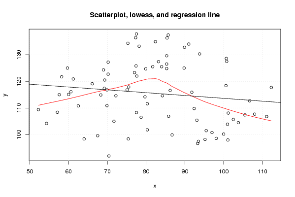
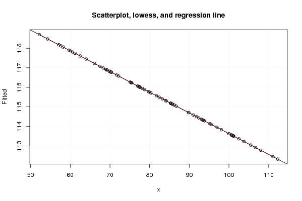
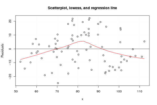
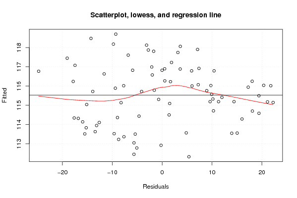
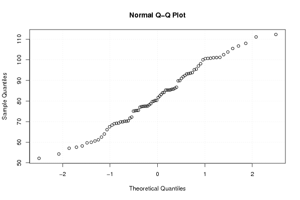
| Title produced by software | Linear Regression Graphical Model Validation | ||||||||||||||||||||||||||||||||||||||||||||||||||||||||||||
| Date of computation | Sat, 10 Nov 2007 03:11:45 -0700 | ||||||||||||||||||||||||||||||||||||||||||||||||||||||||||||
| Cite this page as follows | Statistical Computations at FreeStatistics.org, Office for Research Development and Education, URL https://freestatistics.org/blog/index.php?v=date/2007/Nov/10/t1194689295q05gweix4bodgmq.htm/, Retrieved Tue, 30 Apr 2024 07:02:04 +0000 | ||||||||||||||||||||||||||||||||||||||||||||||||||||||||||||
| Statistical Computations at FreeStatistics.org, Office for Research Development and Education, URL https://freestatistics.org/blog/index.php?pk=4988, Retrieved Tue, 30 Apr 2024 07:02:04 +0000 | |||||||||||||||||||||||||||||||||||||||||||||||||||||||||||||
| QR Codes: | |||||||||||||||||||||||||||||||||||||||||||||||||||||||||||||
|
| |||||||||||||||||||||||||||||||||||||||||||||||||||||||||||||
| Original text written by user: | |||||||||||||||||||||||||||||||||||||||||||||||||||||||||||||
| IsPrivate? | No (this computation is public) | ||||||||||||||||||||||||||||||||||||||||||||||||||||||||||||
| User-defined keywords | 26 duurz vs niet-duurz | ||||||||||||||||||||||||||||||||||||||||||||||||||||||||||||
| Estimated Impact | 231 | ||||||||||||||||||||||||||||||||||||||||||||||||||||||||||||
Tree of Dependent Computations | |||||||||||||||||||||||||||||||||||||||||||||||||||||||||||||
| Family? (F = Feedback message, R = changed R code, M = changed R Module, P = changed Parameters, D = changed Data) | |||||||||||||||||||||||||||||||||||||||||||||||||||||||||||||
| - [Linear Regression Graphical Model Validation] [paper ] [2007-11-10 10:11:45] [8ce1ad2ac57e06e10fb37a1292ae8cb6] [Current] | |||||||||||||||||||||||||||||||||||||||||||||||||||||||||||||
| Feedback Forum | |||||||||||||||||||||||||||||||||||||||||||||||||||||||||||||
Post a new message | |||||||||||||||||||||||||||||||||||||||||||||||||||||||||||||
Dataset | |||||||||||||||||||||||||||||||||||||||||||||||||||||||||||||
| Dataseries X: | |||||||||||||||||||||||||||||||||||||||||||||||||||||||||||||
98.1 101.1 111.1 93.3 100 108 70.4 75.4 105.5 112.3 102.5 93.5 86.7 95.2 103.8 97 95.5 101 67.5 64 106.7 100.6 101.2 93.1 84.2 85.8 91.8 92.4 80.3 79.7 62.5 57.1 100.8 100.7 86.2 83.2 71.7 77.5 89.8 80.3 78.7 93.8 57.6 60.6 91 85.3 77.4 77.3 68.3 69.9 81.7 75.1 69.9 84 54.3 60 89.9 77 85.3 77.6 69.2 75.5 85.7 72.2 79.9 85.3 52.2 61.2 82.4 85.4 78.2 70.2 70.2 69.3 77.5 66.1 69 75.3 58.2 59.7 | |||||||||||||||||||||||||||||||||||||||||||||||||||||||||||||
| Dataseries Y: | |||||||||||||||||||||||||||||||||||||||||||||||||||||||||||||
98,6 98 106,8 96,7 100,2 107,7 92 98,4 107,4 117,7 105,7 97,5 99,9 98,2 104,5 100,8 101,5 103,9 99,6 98,4 112,7 118,4 108,1 105,4 114,6 106,9 115,9 109,8 101,8 114,2 110,8 108,4 127,5 128,6 116,6 127,4 105 108,3 125 111,6 106,5 130,3 115 116,1 134 126,5 125,8 136,4 114,9 110,9 125,5 116,8 116,8 125,5 104,2 115,1 132,8 123,3 124,8 122 117,4 117,9 137,4 114,6 124,7 129,6 109,4 120,9 134,9 136,3 133,2 127,2 122,7 120,5 137,8 119,1 124,3 134,3 121,7 125 | |||||||||||||||||||||||||||||||||||||||||||||||||||||||||||||
Tables (Output of Computation) | |||||||||||||||||||||||||||||||||||||||||||||||||||||||||||||
| |||||||||||||||||||||||||||||||||||||||||||||||||||||||||||||
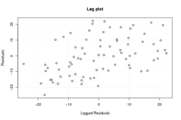
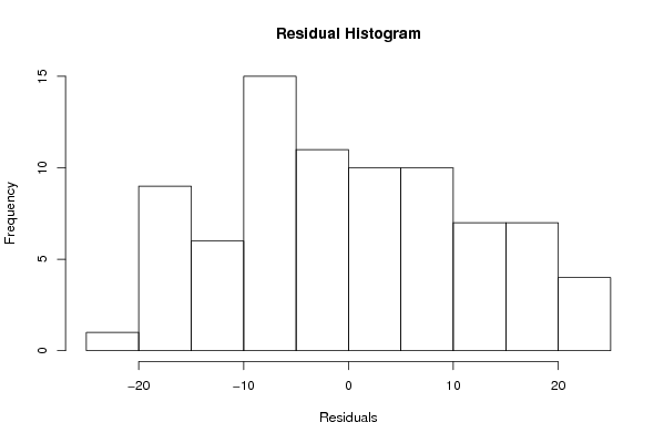
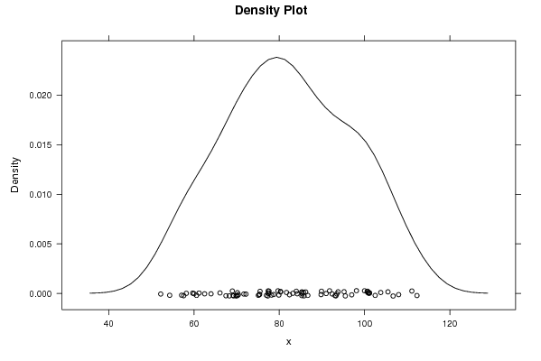
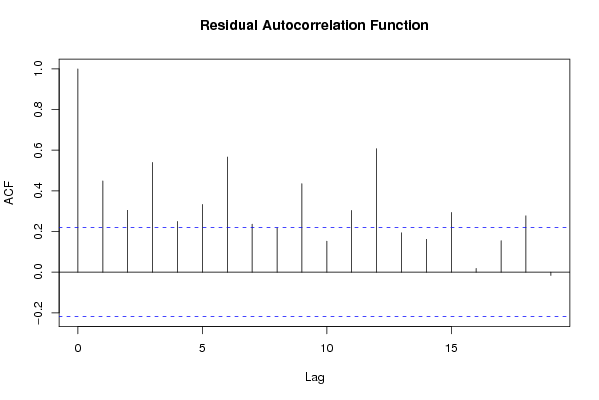
Figures (Output of Computation) | |||||||||||||||||||||||||||||||||||||||||||||||||||||||||||||
Input Parameters & R Code | |||||||||||||||||||||||||||||||||||||||||||||||||||||||||||||
| Parameters (Session): | |||||||||||||||||||||||||||||||||||||||||||||||||||||||||||||
| par1 = 0 ; | |||||||||||||||||||||||||||||||||||||||||||||||||||||||||||||
| Parameters (R input): | |||||||||||||||||||||||||||||||||||||||||||||||||||||||||||||
| par1 = 0 ; | |||||||||||||||||||||||||||||||||||||||||||||||||||||||||||||
| R code (references can be found in the software module): | |||||||||||||||||||||||||||||||||||||||||||||||||||||||||||||
par1 <- as.numeric(par1) | |||||||||||||||||||||||||||||||||||||||||||||||||||||||||||||