Free Statistics
of Irreproducible Research!
Description of Statistical Computation | |||||||||||||||||||||
|---|---|---|---|---|---|---|---|---|---|---|---|---|---|---|---|---|---|---|---|---|---|
| Author's title | |||||||||||||||||||||
| Author | *Unverified author* | ||||||||||||||||||||
| R Software Module | rwasp_meanplot.wasp | ||||||||||||||||||||
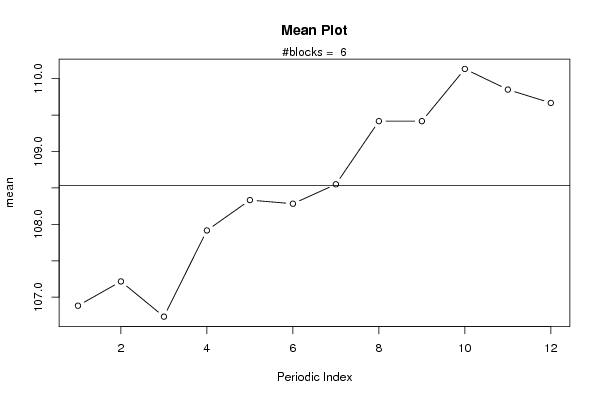
| Title produced by software | Mean Plot | ||||||||||||||||||||
| Date of computation | Thu, 08 Nov 2007 16:19:43 -0700 | ||||||||||||||||||||
| Cite this page as follows | Statistical Computations at FreeStatistics.org, Office for Research Development and Education, URL https://freestatistics.org/blog/index.php?v=date/2007/Nov/09/t1194563912jo8cvyyu7enl2v7.htm/, Retrieved Mon, 06 May 2024 13:59:45 +0000 | ||||||||||||||||||||
| Statistical Computations at FreeStatistics.org, Office for Research Development and Education, URL https://freestatistics.org/blog/index.php?pk=718, Retrieved Mon, 06 May 2024 13:59:45 +0000 | |||||||||||||||||||||
| QR Codes: | |||||||||||||||||||||
|
| |||||||||||||||||||||
| Original text written by user: | |||||||||||||||||||||
| IsPrivate? | No (this computation is public) | ||||||||||||||||||||
| User-defined keywords | |||||||||||||||||||||
| Estimated Impact | 209 | ||||||||||||||||||||
Tree of Dependent Computations | |||||||||||||||||||||
| Family? (F = Feedback message, R = changed R code, M = changed R Module, P = changed Parameters, D = changed Data) | |||||||||||||||||||||
| - [Mean Plot] [Paper 13] [2007-11-08 23:19:43] [640491d00f3c9cca22cbf779aa38ac16] [Current] | |||||||||||||||||||||
| Feedback Forum | |||||||||||||||||||||
Post a new message | |||||||||||||||||||||
Dataset | |||||||||||||||||||||
| Dataseries X: | |||||||||||||||||||||
99,80 103,50 103,10 105,60 105,70 106,60 107,00 105,20 105,70 105,00 105,10 105,90 105,30 104,90 103,20 103,40 104,40 104,50 105,90 110,60 112,40 111,80 111,00 111,00 109,10 107,80 107,20 108,40 107,50 106,40 106,20 104,90 106,20 107,60 107,00 104,50 105,10 104,70 103,70 104,90 105,90 106,10 106,10 106,80 106,40 107,80 107,60 107,60 108,40 109,50 109,20 109,10 110,00 109,00 109,00 111,90 109,30 112,10 112,10 112,50 113,60 112,90 114,00 116,10 116,50 117,10 117,10 117,10 116,50 116,50 116,30 116,50 | |||||||||||||||||||||
Tables (Output of Computation) | |||||||||||||||||||||
| |||||||||||||||||||||
Figures (Output of Computation) | |||||||||||||||||||||
Input Parameters & R Code | |||||||||||||||||||||
| Parameters (Session): | |||||||||||||||||||||
| Parameters (R input): | |||||||||||||||||||||
| par1 = 12 ; | |||||||||||||||||||||
| R code (references can be found in the software module): | |||||||||||||||||||||
par1 <- as.numeric(par1) | |||||||||||||||||||||