Free Statistics
of Irreproducible Research!
Description of Statistical Computation | |||||||||||||||||||||||||||||||||||||
|---|---|---|---|---|---|---|---|---|---|---|---|---|---|---|---|---|---|---|---|---|---|---|---|---|---|---|---|---|---|---|---|---|---|---|---|---|---|
| Author's title | |||||||||||||||||||||||||||||||||||||
| Author | *Unverified author* | ||||||||||||||||||||||||||||||||||||
| R Software Module | rwasp_boxcoxnorm.wasp | ||||||||||||||||||||||||||||||||||||
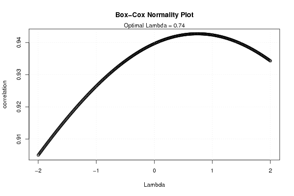
| Title produced by software | Box-Cox Normality Plot | ||||||||||||||||||||||||||||||||||||
| Date of computation | Mon, 05 Nov 2007 04:02:20 -0700 | ||||||||||||||||||||||||||||||||||||
| Cite this page as follows | Statistical Computations at FreeStatistics.org, Office for Research Development and Education, URL https://freestatistics.org/blog/index.php?v=date/2007/Nov/05/us8tkd9yxe7bub01194260467.htm/, Retrieved Sun, 28 Apr 2024 20:09:30 +0000 | ||||||||||||||||||||||||||||||||||||
| Statistical Computations at FreeStatistics.org, Office for Research Development and Education, URL https://freestatistics.org/blog/index.php?pk=528, Retrieved Sun, 28 Apr 2024 20:09:30 +0000 | |||||||||||||||||||||||||||||||||||||
| QR Codes: | |||||||||||||||||||||||||||||||||||||
|
| |||||||||||||||||||||||||||||||||||||
| Original text written by user: | Prijsindexcijfer grondstoffen incl. energie | ||||||||||||||||||||||||||||||||||||
| IsPrivate? | No (this computation is public) | ||||||||||||||||||||||||||||||||||||
| User-defined keywords | |||||||||||||||||||||||||||||||||||||
| Estimated Impact | 208 | ||||||||||||||||||||||||||||||||||||
Tree of Dependent Computations | |||||||||||||||||||||||||||||||||||||
| Family? (F = Feedback message, R = changed R code, M = changed R Module, P = changed Parameters, D = changed Data) | |||||||||||||||||||||||||||||||||||||
| - [Box-Cox Normality Plot] [Q4 WS4 Box Cox No...] [2007-11-05 11:02:20] [4df98167d5cf79c69ce763f2d4ef5b15] [Current] - D [Box-Cox Normality Plot] [Prijsindexcijfer ...] [2008-11-06 16:21:58] [139ab77a283673d78791815259c298e6] | |||||||||||||||||||||||||||||||||||||
| Feedback Forum | |||||||||||||||||||||||||||||||||||||
Post a new message | |||||||||||||||||||||||||||||||||||||
Dataset | |||||||||||||||||||||||||||||||||||||
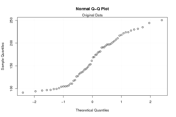
| Dataseries X: | |||||||||||||||||||||||||||||||||||||
96,8 91,2 97,1 104,9 110,9 104,8 94,1 95,8 99,3 101,1 104,0 99,0 105,4 107,1 110,7 117,1 118,7 126,5 127,5 134,6 131,8 135,9 142,7 141,7 153,4 145,0 137,7 148,3 152,2 169,4 168,6 161,1 174,1 179,0 190,6 190,0 181,6 174,8 180,5 196,8 193,8 197,0 216,3 221,4 217,9 229,7 227,4 204,2 196,6 198,8 207,5 190,7 201,6 210,5 223,5 223,8 231,2 244,0 234,7 250,2 | |||||||||||||||||||||||||||||||||||||
Tables (Output of Computation) | |||||||||||||||||||||||||||||||||||||
| |||||||||||||||||||||||||||||||||||||
Figures (Output of Computation) | |||||||||||||||||||||||||||||||||||||
Input Parameters & R Code | |||||||||||||||||||||||||||||||||||||
| Parameters (Session): | |||||||||||||||||||||||||||||||||||||
| Parameters (R input): | |||||||||||||||||||||||||||||||||||||
| R code (references can be found in the software module): | |||||||||||||||||||||||||||||||||||||
n <- length(x) | |||||||||||||||||||||||||||||||||||||