Free Statistics
of Irreproducible Research!
Description of Statistical Computation | |||||||||||||||||||||||||||||||||||||
|---|---|---|---|---|---|---|---|---|---|---|---|---|---|---|---|---|---|---|---|---|---|---|---|---|---|---|---|---|---|---|---|---|---|---|---|---|---|
| Author's title | |||||||||||||||||||||||||||||||||||||
| Author | *Unverified author* | ||||||||||||||||||||||||||||||||||||
| R Software Module | rwasp_boxcoxnorm.wasp | ||||||||||||||||||||||||||||||||||||
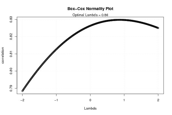
| Title produced by software | Box-Cox Normality Plot | ||||||||||||||||||||||||||||||||||||
| Date of computation | Mon, 05 Nov 2007 09:37:44 -0700 | ||||||||||||||||||||||||||||||||||||
| Cite this page as follows | Statistical Computations at FreeStatistics.org, Office for Research Development and Education, URL https://freestatistics.org/blog/index.php?v=date/2007/Nov/05/rr7d5m2pzz4wuvf1194280553.htm/, Retrieved Mon, 29 Apr 2024 05:45:25 +0000 | ||||||||||||||||||||||||||||||||||||
| Statistical Computations at FreeStatistics.org, Office for Research Development and Education, URL https://freestatistics.org/blog/index.php?pk=516, Retrieved Mon, 29 Apr 2024 05:45:25 +0000 | |||||||||||||||||||||||||||||||||||||
| QR Codes: | |||||||||||||||||||||||||||||||||||||
|
| |||||||||||||||||||||||||||||||||||||
| Original text written by user: | |||||||||||||||||||||||||||||||||||||
| IsPrivate? | No (this computation is public) | ||||||||||||||||||||||||||||||||||||
| User-defined keywords | |||||||||||||||||||||||||||||||||||||
| Estimated Impact | 207 | ||||||||||||||||||||||||||||||||||||
Tree of Dependent Computations | |||||||||||||||||||||||||||||||||||||
| Family? (F = Feedback message, R = changed R code, M = changed R Module, P = changed Parameters, D = changed Data) | |||||||||||||||||||||||||||||||||||||
| - [Box-Cox Normality Plot] [Various EDA Q4] [2007-11-05 16:37:44] [640491d00f3c9cca22cbf779aa38ac16] [Current] | |||||||||||||||||||||||||||||||||||||
| Feedback Forum | |||||||||||||||||||||||||||||||||||||
Post a new message | |||||||||||||||||||||||||||||||||||||
Dataset | |||||||||||||||||||||||||||||||||||||
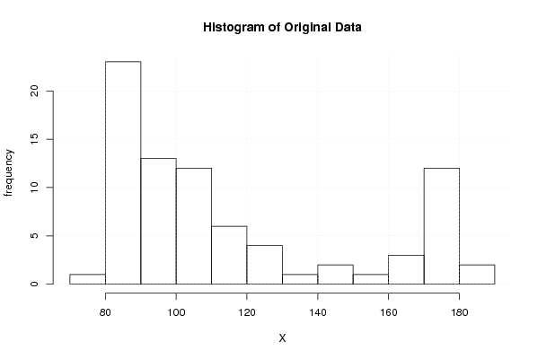
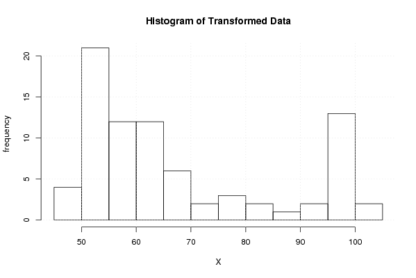
| Dataseries X: | |||||||||||||||||||||||||||||||||||||
100,70 97,90 96,50 96,60 96,60 95,50 91,80 89,30 87,00 85,90 88,00 87,90 89,20 90,90 91,60 90,20 89,10 87,50 86,30 86,00 84,40 86,10 91,00 92,70 88,00 84,30 82,20 80,80 79,40 80,20 82,20 82,20 81,20 82,10 88,10 88,50 92,10 98,60 100,90 100,60 101,10 102,10 103,60 102,80 108,30 104,00 106,10 106,30 109,00 111,00 113,70 112,70 110,30 114,50 119,30 121,80 125,40 129,70 129,40 134,50 141,20 141,40 152,20 167,70 173,30 168,70 172,60 169,80 172,00 179,40 174,60 172,50 172,60 176,30 178,90 179,60 179,90 180,30 180,90 177,70 | |||||||||||||||||||||||||||||||||||||
Tables (Output of Computation) | |||||||||||||||||||||||||||||||||||||
| |||||||||||||||||||||||||||||||||||||
Figures (Output of Computation) | |||||||||||||||||||||||||||||||||||||
Input Parameters & R Code | |||||||||||||||||||||||||||||||||||||
| Parameters (Session): | |||||||||||||||||||||||||||||||||||||
| Parameters (R input): | |||||||||||||||||||||||||||||||||||||
| R code (references can be found in the software module): | |||||||||||||||||||||||||||||||||||||
n <- length(x) | |||||||||||||||||||||||||||||||||||||