Repository of Reproducible Computations

Free Statistics

of Irreproducible Research!

Author's title

Author

*Unverified author*

R Software Module

rwasp_autocorrelation.wasp

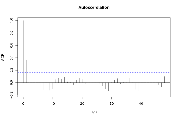
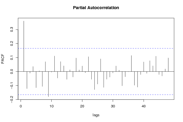
Title produced by software

(Partial) Autocorrelation Function

Date of computation

Thu, 20 Dec 2007 08:39:50 -0700

Cite this page as follows

Statistical Computations at FreeStatistics.org, Office for Research Development and Education, URL https://freestatistics.org/blog/index.php?v=date/2007/Dec/20/t1198164139kwflvd7x99c8tlz.htm/, Retrieved Mon, 29 Apr 2024 08:34:51 +0000

Statistical Computations at FreeStatistics.org, Office for Research Development and Education, URL https://freestatistics.org/blog/index.php?pk=4741, Retrieved Mon, 29 Apr 2024 08:34:51 +0000

QR Codes:

Paste this QR Code to cite your computation.

Original text written by user:

IsPrivate?

No (this computation is public)

User-defined keywords

Estimated Impact

200

Family? (F = Feedback message, R = changed R code, M = changed R Module, P = changed Parameters, D = changed Data)

-       [(Partial) Autocorrelation Function] [partial autocorr ...] [2007-12-20 15:39:50] [8e05505c645e933583b5ad9ab4281af9] [Current]

Feedback Forum

Post a new message

Dataseries X:

Download CSV

Histogram

Boxplots

Summary of compuational transaction
Raw Input	view raw input (R code)
Raw Output	view raw output of R engine
Computing time	3 seconds
R Server	'Herman Ole Andreas Wold' @ 193.190.124.10:1001

\begin{tabular}{lllllllll}
\hline
Summary of compuational transaction \tabularnewline
Raw Input & view raw input (R code)  \tabularnewline
Raw Output & view raw output of R engine  \tabularnewline
Computing time & 3 seconds \tabularnewline
R Server & 'Herman Ole Andreas Wold' @ 193.190.124.10:1001 \tabularnewline
\hline
\end{tabular}
%Source: https://freestatistics.org/blog/index.php?pk=4741&T=0

[TABLE]
[ROW][C]Summary of compuational transaction[/C][/ROW]
[ROW][C]Raw Input[/C][C]view raw input (R code) [/C][/ROW]
[ROW][C]Raw Output[/C][C]view raw output of R engine [/C][/ROW]
[ROW][C]Computing time[/C][C]3 seconds[/C][/ROW]
[ROW][C]R Server[/C][C]'Herman Ole Andreas Wold' @ 193.190.124.10:1001[/C][/ROW]
[/TABLE]
Source: https://freestatistics.org/blog/index.php?pk=4741&T=0

Globally Unique Identifier (entire table): ba.freestatistics.org/blog/index.php?pk=4741&T=0

As an alternative you can also use a QR Code:

The GUIDs for individual cells are displayed in the table below:

Summary of compuational transaction
Raw Input	view raw input (R code)
Raw Output	view raw output of R engine
Computing time	3 seconds
R Server	'Herman Ole Andreas Wold' @ 193.190.124.10:1001

Autocorrelation Function
Time lag k	ACF(k)	T-STAT	P-value
0	1	11.8322	0
1	0.361543	4.2778	1.7e-05
2	0.024565	0.2907	0.385872
3	-0.043699	-0.5171	0.697035
4	0.006266	0.0741	0.470501
5	-0.078834	-0.9328	0.823731
6	-0.066641	-0.7885	0.784132
7	-0.113011	-1.3372	0.908331
8	-0.007844	-0.0928	0.536908
9	-0.122629	-1.451	0.925486
10	-0.102094	-1.208	0.885456
11	0.049026	0.5801	0.281395
12	0.069687	0.8246	0.205514
13	0.054732	0.6476	0.259153
14	0.091499	1.0826	0.140416
15	0.013163	0.1557	0.438228
16	0.001633	0.0193	0.492304
17	-0.032453	-0.384	0.649215
18	0.038355	0.4538	0.325329
19	0.073193	0.866	0.193977
20	0.051444	0.6087	0.271857
21	-0.022947	-0.2715	0.606803
22	0.086011	1.0177	0.155288
23	0.0019	0.0225	0.491049
24	-0.120612	-1.4271	0.922111
25	-0.186221	-2.2034	0.985399
26	-0.01067	-0.1263	0.550143
27	-0.048667	-0.5758	0.717174
28	-0.104134	-1.2321	0.890016
29	-0.130641	-1.5458	0.937791
30	-0.008684	-0.1027	0.540846
31	0.045132	0.534	0.297092
32	0.066399	0.7856	0.216701
33	-0.022558	-0.2669	0.605036
34	0.003031	0.0359	0.485721
35	-0.008827	-0.1044	0.541518
36	0.07595	0.8987	0.185191
37	0.002071	0.0245	0.490244
38	-0.107721	-1.2746	0.897714
39	-0.135189	-1.5996	0.944026
40	0.012024	0.1423	0.443538
41	-0.003355	-0.0397	0.515806
42	0.066948	0.7921	0.214808
43	0.057982	0.686	0.246908
44	0.137176	1.6231	0.05341
45	0.064231	0.76	0.224269
46	-0.032427	-0.3837	0.6491
47	-0.070166	-0.8302	0.796086

\begin{tabular}{lllllllll}
\hline
Autocorrelation Function \tabularnewline
Time lag k & ACF(k) & T-STAT & P-value \tabularnewline
0 & 1 & 11.8322 & 0 \tabularnewline
1 & 0.361543 & 4.2778 & 1.7e-05 \tabularnewline
2 & 0.024565 & 0.2907 & 0.385872 \tabularnewline
3 & -0.043699 & -0.5171 & 0.697035 \tabularnewline
4 & 0.006266 & 0.0741 & 0.470501 \tabularnewline
5 & -0.078834 & -0.9328 & 0.823731 \tabularnewline
6 & -0.066641 & -0.7885 & 0.784132 \tabularnewline
7 & -0.113011 & -1.3372 & 0.908331 \tabularnewline
8 & -0.007844 & -0.0928 & 0.536908 \tabularnewline
9 & -0.122629 & -1.451 & 0.925486 \tabularnewline
10 & -0.102094 & -1.208 & 0.885456 \tabularnewline
11 & 0.049026 & 0.5801 & 0.281395 \tabularnewline
12 & 0.069687 & 0.8246 & 0.205514 \tabularnewline
13 & 0.054732 & 0.6476 & 0.259153 \tabularnewline
14 & 0.091499 & 1.0826 & 0.140416 \tabularnewline
15 & 0.013163 & 0.1557 & 0.438228 \tabularnewline
16 & 0.001633 & 0.0193 & 0.492304 \tabularnewline
17 & -0.032453 & -0.384 & 0.649215 \tabularnewline
18 & 0.038355 & 0.4538 & 0.325329 \tabularnewline
19 & 0.073193 & 0.866 & 0.193977 \tabularnewline
20 & 0.051444 & 0.6087 & 0.271857 \tabularnewline
21 & -0.022947 & -0.2715 & 0.606803 \tabularnewline
22 & 0.086011 & 1.0177 & 0.155288 \tabularnewline
23 & 0.0019 & 0.0225 & 0.491049 \tabularnewline
24 & -0.120612 & -1.4271 & 0.922111 \tabularnewline
25 & -0.186221 & -2.2034 & 0.985399 \tabularnewline
26 & -0.01067 & -0.1263 & 0.550143 \tabularnewline
27 & -0.048667 & -0.5758 & 0.717174 \tabularnewline
28 & -0.104134 & -1.2321 & 0.890016 \tabularnewline
29 & -0.130641 & -1.5458 & 0.937791 \tabularnewline
30 & -0.008684 & -0.1027 & 0.540846 \tabularnewline
31 & 0.045132 & 0.534 & 0.297092 \tabularnewline
32 & 0.066399 & 0.7856 & 0.216701 \tabularnewline
33 & -0.022558 & -0.2669 & 0.605036 \tabularnewline
34 & 0.003031 & 0.0359 & 0.485721 \tabularnewline
35 & -0.008827 & -0.1044 & 0.541518 \tabularnewline
36 & 0.07595 & 0.8987 & 0.185191 \tabularnewline
37 & 0.002071 & 0.0245 & 0.490244 \tabularnewline
38 & -0.107721 & -1.2746 & 0.897714 \tabularnewline
39 & -0.135189 & -1.5996 & 0.944026 \tabularnewline
40 & 0.012024 & 0.1423 & 0.443538 \tabularnewline
41 & -0.003355 & -0.0397 & 0.515806 \tabularnewline
42 & 0.066948 & 0.7921 & 0.214808 \tabularnewline
43 & 0.057982 & 0.686 & 0.246908 \tabularnewline
44 & 0.137176 & 1.6231 & 0.05341 \tabularnewline
45 & 0.064231 & 0.76 & 0.224269 \tabularnewline
46 & -0.032427 & -0.3837 & 0.6491 \tabularnewline
47 & -0.070166 & -0.8302 & 0.796086 \tabularnewline
\hline
\end{tabular}
%Source: https://freestatistics.org/blog/index.php?pk=4741&T=1

[TABLE]
[ROW][C]Autocorrelation Function[/C][/ROW]
[ROW][C]Time lag k[/C][C]ACF(k)[/C][C]T-STAT[/C][C]P-value[/C][/ROW]
[ROW][C]0[/C][C]1[/C][C]11.8322[/C][C]0[/C][/ROW]
[ROW][C]1[/C][C]0.361543[/C][C]4.2778[/C][C]1.7e-05[/C][/ROW]
[ROW][C]2[/C][C]0.024565[/C][C]0.2907[/C][C]0.385872[/C][/ROW]
[ROW][C]3[/C][C]-0.043699[/C][C]-0.5171[/C][C]0.697035[/C][/ROW]
[ROW][C]4[/C][C]0.006266[/C][C]0.0741[/C][C]0.470501[/C][/ROW]
[ROW][C]5[/C][C]-0.078834[/C][C]-0.9328[/C][C]0.823731[/C][/ROW]
[ROW][C]6[/C][C]-0.066641[/C][C]-0.7885[/C][C]0.784132[/C][/ROW]
[ROW][C]7[/C][C]-0.113011[/C][C]-1.3372[/C][C]0.908331[/C][/ROW]
[ROW][C]8[/C][C]-0.007844[/C][C]-0.0928[/C][C]0.536908[/C][/ROW]
[ROW][C]9[/C][C]-0.122629[/C][C]-1.451[/C][C]0.925486[/C][/ROW]
[ROW][C]10[/C][C]-0.102094[/C][C]-1.208[/C][C]0.885456[/C][/ROW]
[ROW][C]11[/C][C]0.049026[/C][C]0.5801[/C][C]0.281395[/C][/ROW]
[ROW][C]12[/C][C]0.069687[/C][C]0.8246[/C][C]0.205514[/C][/ROW]
[ROW][C]13[/C][C]0.054732[/C][C]0.6476[/C][C]0.259153[/C][/ROW]
[ROW][C]14[/C][C]0.091499[/C][C]1.0826[/C][C]0.140416[/C][/ROW]
[ROW][C]15[/C][C]0.013163[/C][C]0.1557[/C][C]0.438228[/C][/ROW]
[ROW][C]16[/C][C]0.001633[/C][C]0.0193[/C][C]0.492304[/C][/ROW]
[ROW][C]17[/C][C]-0.032453[/C][C]-0.384[/C][C]0.649215[/C][/ROW]
[ROW][C]18[/C][C]0.038355[/C][C]0.4538[/C][C]0.325329[/C][/ROW]
[ROW][C]19[/C][C]0.073193[/C][C]0.866[/C][C]0.193977[/C][/ROW]
[ROW][C]20[/C][C]0.051444[/C][C]0.6087[/C][C]0.271857[/C][/ROW]
[ROW][C]21[/C][C]-0.022947[/C][C]-0.2715[/C][C]0.606803[/C][/ROW]
[ROW][C]22[/C][C]0.086011[/C][C]1.0177[/C][C]0.155288[/C][/ROW]
[ROW][C]23[/C][C]0.0019[/C][C]0.0225[/C][C]0.491049[/C][/ROW]
[ROW][C]24[/C][C]-0.120612[/C][C]-1.4271[/C][C]0.922111[/C][/ROW]
[ROW][C]25[/C][C]-0.186221[/C][C]-2.2034[/C][C]0.985399[/C][/ROW]
[ROW][C]26[/C][C]-0.01067[/C][C]-0.1263[/C][C]0.550143[/C][/ROW]
[ROW][C]27[/C][C]-0.048667[/C][C]-0.5758[/C][C]0.717174[/C][/ROW]
[ROW][C]28[/C][C]-0.104134[/C][C]-1.2321[/C][C]0.890016[/C][/ROW]
[ROW][C]29[/C][C]-0.130641[/C][C]-1.5458[/C][C]0.937791[/C][/ROW]
[ROW][C]30[/C][C]-0.008684[/C][C]-0.1027[/C][C]0.540846[/C][/ROW]
[ROW][C]31[/C][C]0.045132[/C][C]0.534[/C][C]0.297092[/C][/ROW]
[ROW][C]32[/C][C]0.066399[/C][C]0.7856[/C][C]0.216701[/C][/ROW]
[ROW][C]33[/C][C]-0.022558[/C][C]-0.2669[/C][C]0.605036[/C][/ROW]
[ROW][C]34[/C][C]0.003031[/C][C]0.0359[/C][C]0.485721[/C][/ROW]
[ROW][C]35[/C][C]-0.008827[/C][C]-0.1044[/C][C]0.541518[/C][/ROW]
[ROW][C]36[/C][C]0.07595[/C][C]0.8987[/C][C]0.185191[/C][/ROW]
[ROW][C]37[/C][C]0.002071[/C][C]0.0245[/C][C]0.490244[/C][/ROW]
[ROW][C]38[/C][C]-0.107721[/C][C]-1.2746[/C][C]0.897714[/C][/ROW]
[ROW][C]39[/C][C]-0.135189[/C][C]-1.5996[/C][C]0.944026[/C][/ROW]
[ROW][C]40[/C][C]0.012024[/C][C]0.1423[/C][C]0.443538[/C][/ROW]
[ROW][C]41[/C][C]-0.003355[/C][C]-0.0397[/C][C]0.515806[/C][/ROW]
[ROW][C]42[/C][C]0.066948[/C][C]0.7921[/C][C]0.214808[/C][/ROW]
[ROW][C]43[/C][C]0.057982[/C][C]0.686[/C][C]0.246908[/C][/ROW]
[ROW][C]44[/C][C]0.137176[/C][C]1.6231[/C][C]0.05341[/C][/ROW]
[ROW][C]45[/C][C]0.064231[/C][C]0.76[/C][C]0.224269[/C][/ROW]
[ROW][C]46[/C][C]-0.032427[/C][C]-0.3837[/C][C]0.6491[/C][/ROW]
[ROW][C]47[/C][C]-0.070166[/C][C]-0.8302[/C][C]0.796086[/C][/ROW]
[/TABLE]
Source: https://freestatistics.org/blog/index.php?pk=4741&T=1

Globally Unique Identifier (entire table): ba.freestatistics.org/blog/index.php?pk=4741&T=1

As an alternative you can also use a QR Code:

The GUIDs for individual cells are displayed in the table below:

Autocorrelation Function
Time lag k	ACF(k)	T-STAT	P-value
0	1	11.8322	0
1	0.361543	4.2778	1.7e-05
2	0.024565	0.2907	0.385872
3	-0.043699	-0.5171	0.697035
4	0.006266	0.0741	0.470501
5	-0.078834	-0.9328	0.823731
6	-0.066641	-0.7885	0.784132
7	-0.113011	-1.3372	0.908331
8	-0.007844	-0.0928	0.536908
9	-0.122629	-1.451	0.925486
10	-0.102094	-1.208	0.885456
11	0.049026	0.5801	0.281395
12	0.069687	0.8246	0.205514
13	0.054732	0.6476	0.259153
14	0.091499	1.0826	0.140416
15	0.013163	0.1557	0.438228
16	0.001633	0.0193	0.492304
17	-0.032453	-0.384	0.649215
18	0.038355	0.4538	0.325329
19	0.073193	0.866	0.193977
20	0.051444	0.6087	0.271857
21	-0.022947	-0.2715	0.606803
22	0.086011	1.0177	0.155288
23	0.0019	0.0225	0.491049
24	-0.120612	-1.4271	0.922111
25	-0.186221	-2.2034	0.985399
26	-0.01067	-0.1263	0.550143
27	-0.048667	-0.5758	0.717174
28	-0.104134	-1.2321	0.890016
29	-0.130641	-1.5458	0.937791
30	-0.008684	-0.1027	0.540846
31	0.045132	0.534	0.297092
32	0.066399	0.7856	0.216701
33	-0.022558	-0.2669	0.605036
34	0.003031	0.0359	0.485721
35	-0.008827	-0.1044	0.541518
36	0.07595	0.8987	0.185191
37	0.002071	0.0245	0.490244
38	-0.107721	-1.2746	0.897714
39	-0.135189	-1.5996	0.944026
40	0.012024	0.1423	0.443538
41	-0.003355	-0.0397	0.515806
42	0.066948	0.7921	0.214808
43	0.057982	0.686	0.246908
44	0.137176	1.6231	0.05341
45	0.064231	0.76	0.224269
46	-0.032427	-0.3837	0.6491
47	-0.070166	-0.8302	0.796086

Partial Autocorrelation Function
Time lag k	PACF(k)	T-STAT	P-value
0	0.361543	4.2778	1.7e-05
1	-0.12211	-1.4448	0.924629
2	-0.011114	-0.1315	0.552217
3	0.036022	0.4262	0.335303
4	-0.115444	-1.366	0.912928
5	0.005137	0.0608	0.475808
6	-0.10669	-1.2624	0.895542
7	0.070418	0.8332	0.203078
8	-0.17918	-2.1201	0.982119
9	-0.004324	-0.0512	0.520364
10	0.111058	1.3141	0.095489
11	-0.046778	-0.5535	0.709591
12	0.071299	0.8436	0.20016
13	0.040549	0.4798	0.316064
14	-0.056044	-0.6631	0.74583
15	0.012663	0.1498	0.440559
16	-0.03889	-0.4602	0.67694
17	0.096493	1.1417	0.127759
18	0.011872	0.1405	0.444243
19	0.039515	0.4676	0.320416
20	-0.008443	-0.0999	0.539718
21	0.106233	1.257	0.105431
22	-0.055659	-0.6586	0.744371
23	-0.129075	-1.5272	0.93552
24	-0.089721	-1.0616	0.854875
25	0.090557	1.0715	0.142898
26	-0.113493	-1.3429	0.909257
27	-0.054996	-0.6507	0.741855
28	-0.039704	-0.4698	0.680379
29	-0.010115	-0.1197	0.547546
30	0.039773	0.4706	0.319328
31	0.009936	0.1176	0.453289
32	-0.102078	-1.2078	0.88542
33	-0.037497	-0.4437	0.671019
34	-0.001002	-0.0119	0.504722
35	0.114683	1.3569	0.088491
36	-0.097996	-1.1595	0.875888
37	-0.111591	-1.3204	0.905565
38	-0.021605	-0.2556	0.600696
39	0.068866	0.8148	0.208277
40	-0.013055	-0.1545	0.561269
41	0.077618	0.9184	0.179998
42	0.040705	0.4816	0.315412
43	0.110012	1.3017	0.097581
44	-0.02134	-0.2525	0.599487
45	-0.031619	-0.3741	0.645562
46	0.018472	0.2186	0.413654
47	0.097402	1.1525	0.125546

\begin{tabular}{lllllllll}
\hline
Partial Autocorrelation Function \tabularnewline
Time lag k & PACF(k) & T-STAT & P-value \tabularnewline
0 & 0.361543 & 4.2778 & 1.7e-05 \tabularnewline
1 & -0.12211 & -1.4448 & 0.924629 \tabularnewline
2 & -0.011114 & -0.1315 & 0.552217 \tabularnewline
3 & 0.036022 & 0.4262 & 0.335303 \tabularnewline
4 & -0.115444 & -1.366 & 0.912928 \tabularnewline
5 & 0.005137 & 0.0608 & 0.475808 \tabularnewline
6 & -0.10669 & -1.2624 & 0.895542 \tabularnewline
7 & 0.070418 & 0.8332 & 0.203078 \tabularnewline
8 & -0.17918 & -2.1201 & 0.982119 \tabularnewline
9 & -0.004324 & -0.0512 & 0.520364 \tabularnewline
10 & 0.111058 & 1.3141 & 0.095489 \tabularnewline
11 & -0.046778 & -0.5535 & 0.709591 \tabularnewline
12 & 0.071299 & 0.8436 & 0.20016 \tabularnewline
13 & 0.040549 & 0.4798 & 0.316064 \tabularnewline
14 & -0.056044 & -0.6631 & 0.74583 \tabularnewline
15 & 0.012663 & 0.1498 & 0.440559 \tabularnewline
16 & -0.03889 & -0.4602 & 0.67694 \tabularnewline
17 & 0.096493 & 1.1417 & 0.127759 \tabularnewline
18 & 0.011872 & 0.1405 & 0.444243 \tabularnewline
19 & 0.039515 & 0.4676 & 0.320416 \tabularnewline
20 & -0.008443 & -0.0999 & 0.539718 \tabularnewline
21 & 0.106233 & 1.257 & 0.105431 \tabularnewline
22 & -0.055659 & -0.6586 & 0.744371 \tabularnewline
23 & -0.129075 & -1.5272 & 0.93552 \tabularnewline
24 & -0.089721 & -1.0616 & 0.854875 \tabularnewline
25 & 0.090557 & 1.0715 & 0.142898 \tabularnewline
26 & -0.113493 & -1.3429 & 0.909257 \tabularnewline
27 & -0.054996 & -0.6507 & 0.741855 \tabularnewline
28 & -0.039704 & -0.4698 & 0.680379 \tabularnewline
29 & -0.010115 & -0.1197 & 0.547546 \tabularnewline
30 & 0.039773 & 0.4706 & 0.319328 \tabularnewline
31 & 0.009936 & 0.1176 & 0.453289 \tabularnewline
32 & -0.102078 & -1.2078 & 0.88542 \tabularnewline
33 & -0.037497 & -0.4437 & 0.671019 \tabularnewline
34 & -0.001002 & -0.0119 & 0.504722 \tabularnewline
35 & 0.114683 & 1.3569 & 0.088491 \tabularnewline
36 & -0.097996 & -1.1595 & 0.875888 \tabularnewline
37 & -0.111591 & -1.3204 & 0.905565 \tabularnewline
38 & -0.021605 & -0.2556 & 0.600696 \tabularnewline
39 & 0.068866 & 0.8148 & 0.208277 \tabularnewline
40 & -0.013055 & -0.1545 & 0.561269 \tabularnewline
41 & 0.077618 & 0.9184 & 0.179998 \tabularnewline
42 & 0.040705 & 0.4816 & 0.315412 \tabularnewline
43 & 0.110012 & 1.3017 & 0.097581 \tabularnewline
44 & -0.02134 & -0.2525 & 0.599487 \tabularnewline
45 & -0.031619 & -0.3741 & 0.645562 \tabularnewline
46 & 0.018472 & 0.2186 & 0.413654 \tabularnewline
47 & 0.097402 & 1.1525 & 0.125546 \tabularnewline
\hline
\end{tabular}
%Source: https://freestatistics.org/blog/index.php?pk=4741&T=2

[TABLE]
[ROW][C]Partial Autocorrelation Function[/C][/ROW]
[ROW][C]Time lag k[/C][C]PACF(k)[/C][C]T-STAT[/C][C]P-value[/C][/ROW]
[ROW][C]0[/C][C]0.361543[/C][C]4.2778[/C][C]1.7e-05[/C][/ROW]
[ROW][C]1[/C][C]-0.12211[/C][C]-1.4448[/C][C]0.924629[/C][/ROW]
[ROW][C]2[/C][C]-0.011114[/C][C]-0.1315[/C][C]0.552217[/C][/ROW]
[ROW][C]3[/C][C]0.036022[/C][C]0.4262[/C][C]0.335303[/C][/ROW]
[ROW][C]4[/C][C]-0.115444[/C][C]-1.366[/C][C]0.912928[/C][/ROW]
[ROW][C]5[/C][C]0.005137[/C][C]0.0608[/C][C]0.475808[/C][/ROW]
[ROW][C]6[/C][C]-0.10669[/C][C]-1.2624[/C][C]0.895542[/C][/ROW]
[ROW][C]7[/C][C]0.070418[/C][C]0.8332[/C][C]0.203078[/C][/ROW]
[ROW][C]8[/C][C]-0.17918[/C][C]-2.1201[/C][C]0.982119[/C][/ROW]
[ROW][C]9[/C][C]-0.004324[/C][C]-0.0512[/C][C]0.520364[/C][/ROW]
[ROW][C]10[/C][C]0.111058[/C][C]1.3141[/C][C]0.095489[/C][/ROW]
[ROW][C]11[/C][C]-0.046778[/C][C]-0.5535[/C][C]0.709591[/C][/ROW]
[ROW][C]12[/C][C]0.071299[/C][C]0.8436[/C][C]0.20016[/C][/ROW]
[ROW][C]13[/C][C]0.040549[/C][C]0.4798[/C][C]0.316064[/C][/ROW]
[ROW][C]14[/C][C]-0.056044[/C][C]-0.6631[/C][C]0.74583[/C][/ROW]
[ROW][C]15[/C][C]0.012663[/C][C]0.1498[/C][C]0.440559[/C][/ROW]
[ROW][C]16[/C][C]-0.03889[/C][C]-0.4602[/C][C]0.67694[/C][/ROW]
[ROW][C]17[/C][C]0.096493[/C][C]1.1417[/C][C]0.127759[/C][/ROW]
[ROW][C]18[/C][C]0.011872[/C][C]0.1405[/C][C]0.444243[/C][/ROW]
[ROW][C]19[/C][C]0.039515[/C][C]0.4676[/C][C]0.320416[/C][/ROW]
[ROW][C]20[/C][C]-0.008443[/C][C]-0.0999[/C][C]0.539718[/C][/ROW]
[ROW][C]21[/C][C]0.106233[/C][C]1.257[/C][C]0.105431[/C][/ROW]
[ROW][C]22[/C][C]-0.055659[/C][C]-0.6586[/C][C]0.744371[/C][/ROW]
[ROW][C]23[/C][C]-0.129075[/C][C]-1.5272[/C][C]0.93552[/C][/ROW]
[ROW][C]24[/C][C]-0.089721[/C][C]-1.0616[/C][C]0.854875[/C][/ROW]
[ROW][C]25[/C][C]0.090557[/C][C]1.0715[/C][C]0.142898[/C][/ROW]
[ROW][C]26[/C][C]-0.113493[/C][C]-1.3429[/C][C]0.909257[/C][/ROW]
[ROW][C]27[/C][C]-0.054996[/C][C]-0.6507[/C][C]0.741855[/C][/ROW]
[ROW][C]28[/C][C]-0.039704[/C][C]-0.4698[/C][C]0.680379[/C][/ROW]
[ROW][C]29[/C][C]-0.010115[/C][C]-0.1197[/C][C]0.547546[/C][/ROW]
[ROW][C]30[/C][C]0.039773[/C][C]0.4706[/C][C]0.319328[/C][/ROW]
[ROW][C]31[/C][C]0.009936[/C][C]0.1176[/C][C]0.453289[/C][/ROW]
[ROW][C]32[/C][C]-0.102078[/C][C]-1.2078[/C][C]0.88542[/C][/ROW]
[ROW][C]33[/C][C]-0.037497[/C][C]-0.4437[/C][C]0.671019[/C][/ROW]
[ROW][C]34[/C][C]-0.001002[/C][C]-0.0119[/C][C]0.504722[/C][/ROW]
[ROW][C]35[/C][C]0.114683[/C][C]1.3569[/C][C]0.088491[/C][/ROW]
[ROW][C]36[/C][C]-0.097996[/C][C]-1.1595[/C][C]0.875888[/C][/ROW]
[ROW][C]37[/C][C]-0.111591[/C][C]-1.3204[/C][C]0.905565[/C][/ROW]
[ROW][C]38[/C][C]-0.021605[/C][C]-0.2556[/C][C]0.600696[/C][/ROW]
[ROW][C]39[/C][C]0.068866[/C][C]0.8148[/C][C]0.208277[/C][/ROW]
[ROW][C]40[/C][C]-0.013055[/C][C]-0.1545[/C][C]0.561269[/C][/ROW]
[ROW][C]41[/C][C]0.077618[/C][C]0.9184[/C][C]0.179998[/C][/ROW]
[ROW][C]42[/C][C]0.040705[/C][C]0.4816[/C][C]0.315412[/C][/ROW]
[ROW][C]43[/C][C]0.110012[/C][C]1.3017[/C][C]0.097581[/C][/ROW]
[ROW][C]44[/C][C]-0.02134[/C][C]-0.2525[/C][C]0.599487[/C][/ROW]
[ROW][C]45[/C][C]-0.031619[/C][C]-0.3741[/C][C]0.645562[/C][/ROW]
[ROW][C]46[/C][C]0.018472[/C][C]0.2186[/C][C]0.413654[/C][/ROW]
[ROW][C]47[/C][C]0.097402[/C][C]1.1525[/C][C]0.125546[/C][/ROW]
[/TABLE]
Source: https://freestatistics.org/blog/index.php?pk=4741&T=2

Globally Unique Identifier (entire table): ba.freestatistics.org/blog/index.php?pk=4741&T=2

As an alternative you can also use a QR Code:

The GUIDs for individual cells are displayed in the table below:

Partial Autocorrelation Function
Time lag k	PACF(k)	T-STAT	P-value
0	0.361543	4.2778	1.7e-05
1	-0.12211	-1.4448	0.924629
2	-0.011114	-0.1315	0.552217
3	0.036022	0.4262	0.335303
4	-0.115444	-1.366	0.912928
5	0.005137	0.0608	0.475808
6	-0.10669	-1.2624	0.895542
7	0.070418	0.8332	0.203078
8	-0.17918	-2.1201	0.982119
9	-0.004324	-0.0512	0.520364
10	0.111058	1.3141	0.095489
11	-0.046778	-0.5535	0.709591
12	0.071299	0.8436	0.20016
13	0.040549	0.4798	0.316064
14	-0.056044	-0.6631	0.74583
15	0.012663	0.1498	0.440559
16	-0.03889	-0.4602	0.67694
17	0.096493	1.1417	0.127759
18	0.011872	0.1405	0.444243
19	0.039515	0.4676	0.320416
20	-0.008443	-0.0999	0.539718
21	0.106233	1.257	0.105431
22	-0.055659	-0.6586	0.744371
23	-0.129075	-1.5272	0.93552
24	-0.089721	-1.0616	0.854875
25	0.090557	1.0715	0.142898
26	-0.113493	-1.3429	0.909257
27	-0.054996	-0.6507	0.741855
28	-0.039704	-0.4698	0.680379
29	-0.010115	-0.1197	0.547546
30	0.039773	0.4706	0.319328
31	0.009936	0.1176	0.453289
32	-0.102078	-1.2078	0.88542
33	-0.037497	-0.4437	0.671019
34	-0.001002	-0.0119	0.504722
35	0.114683	1.3569	0.088491
36	-0.097996	-1.1595	0.875888
37	-0.111591	-1.3204	0.905565
38	-0.021605	-0.2556	0.600696
39	0.068866	0.8148	0.208277
40	-0.013055	-0.1545	0.561269
41	0.077618	0.9184	0.179998
42	0.040705	0.4816	0.315412
43	0.110012	1.3017	0.097581
44	-0.02134	-0.2525	0.599487
45	-0.031619	-0.3741	0.645562
46	0.018472	0.2186	0.413654
47	0.097402	1.1525	0.125546

Figure 1

PNG link

Postscript link

PDF link

Figure 2

PNG link

Postscript link

PDF link

Parameters (Session):

par1 = 48 ; par2 = 0.0 ; par3 = 1 ; par4 = 0 ; par5 = 12 ;

Parameters (R input):

par1 = 48 ; par2 = 0.0 ; par3 = 1 ; par4 = 0 ; par5 = 12 ;

R code (references can be found in the software module):

if (par1 == 'Default') {
par1 = 10*log10(length(x))
} else {
par1 <- as.numeric(par1)
}
par2 <- as.numeric(par2)
par3 <- as.numeric(par3)
par4 <- as.numeric(par4)
par5 <- as.numeric(par5)
if (par2 == 0) {
x <- log(x)
} else {
x <- (x ^ par2 - 1) / par2
}
if (par3 > 0) x <- diff(x,lag=1,difference=par3)
if (par4 > 0) x <- diff(x,lag=par5,difference=par4)
bitmap(file='pic1.png')
racf <- acf(x,par1,main='Autocorrelation',xlab='lags',ylab='ACF')
dev.off()
bitmap(file='pic2.png')
rpacf <- pacf(x,par1,main='Partial Autocorrelation',xlab='lags',ylab='PACF')
dev.off()
(myacf <- c(racf$acf))
(mypacf <- c(rpacf$acf))
lengthx <- length(x)
sqrtn <- sqrt(lengthx)
load(file='createtable')
a<-table.start()
a<-table.row.start(a)
a<-table.element(a,'Autocorrelation Function',4,TRUE)
a<-table.row.end(a)
a<-table.row.start(a)
a<-table.element(a,'Time lag k',header=TRUE)
a<-table.element(a,hyperlink('basics.htm','ACF(k)','click here for more information about the Autocorrelation Function'),header=TRUE)
a<-table.element(a,'T-STAT',header=TRUE)
a<-table.element(a,'P-value',header=TRUE)
a<-table.row.end(a)
for (i in 1:par1) {
a<-table.row.start(a)
a<-table.element(a,i-1,header=TRUE)
a<-table.element(a,round(myacf[i],6))
mytstat <- myacf[i]*sqrtn
a<-table.element(a,round(mytstat,4))
a<-table.element(a,round(1-pt(mytstat,lengthx),6))
a<-table.row.end(a)
}
a<-table.end(a)
table.save(a,file='mytable.tab')
a<-table.start()
a<-table.row.start(a)
a<-table.element(a,'Partial Autocorrelation Function',4,TRUE)
a<-table.row.end(a)
a<-table.row.start(a)
a<-table.element(a,'Time lag k',header=TRUE)
a<-table.element(a,hyperlink('basics.htm','PACF(k)','click here for more information about the Partial Autocorrelation Function'),header=TRUE)
a<-table.element(a,'T-STAT',header=TRUE)
a<-table.element(a,'P-value',header=TRUE)
a<-table.row.end(a)
for (i in 1:par1) {
a<-table.row.start(a)
a<-table.element(a,i-1,header=TRUE)
a<-table.element(a,round(mypacf[i],6))
mytstat <- mypacf[i]*sqrtn
a<-table.element(a,round(mytstat,4))
a<-table.element(a,round(1-pt(mytstat,lengthx),6))
a<-table.row.end(a)
}
a<-table.end(a)
table.save(a,file='mytable1.tab')

Free Statistics

Description of Statistical Computation

Tree of Dependent Computations

Dataset

Tables (Output of Computation)

Figures (Output of Computation)

Input Parameters & R Code