Repository of Reproducible Computations

Free Statistics

of Irreproducible Research!

Author's title

Author

*Unverified author*

R Software Module

rwasp_autocorrelation.wasp

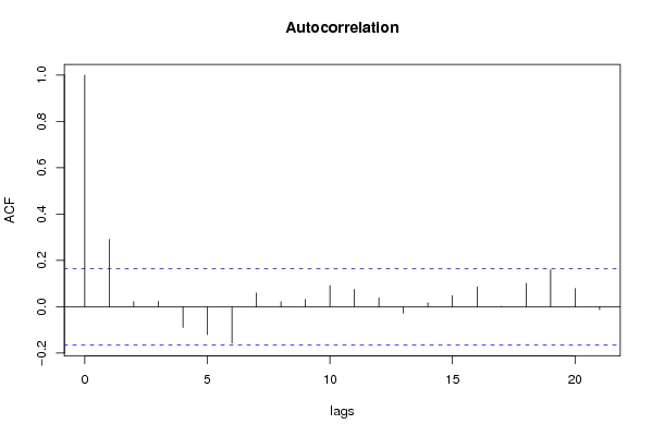
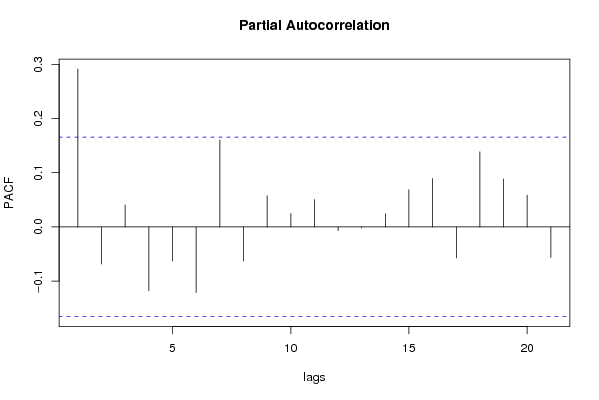
Title produced by software

(Partial) Autocorrelation Function

Date of computation

Thu, 20 Dec 2007 08:34:39 -0700

Cite this page as follows

Statistical Computations at FreeStatistics.org, Office for Research Development and Education, URL https://freestatistics.org/blog/index.php?v=date/2007/Dec/20/t1198163804iuze2h1yvuctxuz.htm/, Retrieved Mon, 29 Apr 2024 11:31:13 +0000

Statistical Computations at FreeStatistics.org, Office for Research Development and Education, URL https://freestatistics.org/blog/index.php?pk=4738, Retrieved Mon, 29 Apr 2024 11:31:13 +0000

QR Codes:

Paste this QR Code to cite your computation.

Original text written by user:

IsPrivate?

No (this computation is public)

User-defined keywords

Estimated Impact

211

Family? (F = Feedback message, R = changed R code, M = changed R Module, P = changed Parameters, D = changed Data)

-       [(Partial) Autocorrelation Function] [partial autocorr ...] [2007-12-20 15:34:39] [8e05505c645e933583b5ad9ab4281af9] [Current]

Feedback Forum

Post a new message

Dataseries X:

Download CSV

Histogram

Boxplots

Summary of compuational transaction
Raw Input	view raw input (R code)
Raw Output	view raw output of R engine
Computing time	1 seconds
R Server	'Gwilym Jenkins' @ 72.249.127.135

\begin{tabular}{lllllllll}
\hline
Summary of compuational transaction \tabularnewline
Raw Input & view raw input (R code)  \tabularnewline
Raw Output & view raw output of R engine  \tabularnewline
Computing time & 1 seconds \tabularnewline
R Server & 'Gwilym Jenkins' @ 72.249.127.135 \tabularnewline
\hline
\end{tabular}
%Source: https://freestatistics.org/blog/index.php?pk=4738&T=0

[TABLE]
[ROW][C]Summary of compuational transaction[/C][/ROW]
[ROW][C]Raw Input[/C][C]view raw input (R code) [/C][/ROW]
[ROW][C]Raw Output[/C][C]view raw output of R engine [/C][/ROW]
[ROW][C]Computing time[/C][C]1 seconds[/C][/ROW]
[ROW][C]R Server[/C][C]'Gwilym Jenkins' @ 72.249.127.135[/C][/ROW]
[/TABLE]
Source: https://freestatistics.org/blog/index.php?pk=4738&T=0

Globally Unique Identifier (entire table): ba.freestatistics.org/blog/index.php?pk=4738&T=0

As an alternative you can also use a QR Code:

The GUIDs for individual cells are displayed in the table below:

Summary of compuational transaction
Raw Input	view raw input (R code)
Raw Output	view raw output of R engine
Computing time	1 seconds
R Server	'Gwilym Jenkins' @ 72.249.127.135

Autocorrelation Function
Time lag k	ACF(k)	T-STAT	P-value
0	1	11.8322	0
1	0.291526	3.4494	0.000371
2	0.022126	0.2618	0.396931
3	0.023829	0.2819	0.389201
4	-0.08951	-1.0591	0.854311
5	-0.119855	-1.4181	0.920815
6	-0.156509	-1.8518	0.966922
7	0.059759	0.7071	0.240345
8	0.02176	0.2575	0.398598
9	0.032108	0.3799	0.352295
10	0.091074	1.0776	0.141533
11	0.075395	0.8921	0.186939
12	0.039014	0.4616	0.322535
13	-0.027386	-0.324	0.626804
14	0.017319	0.2049	0.418967
15	0.048087	0.569	0.285143
16	0.085968	1.0172	0.155409
17	0.002556	0.0302	0.487956
18	0.10112	1.1965	0.116769
19	0.15965	1.889	0.03048
20	0.07909	0.9358	0.175492

\begin{tabular}{lllllllll}
\hline
Autocorrelation Function \tabularnewline
Time lag k & ACF(k) & T-STAT & P-value \tabularnewline
0 & 1 & 11.8322 & 0 \tabularnewline
1 & 0.291526 & 3.4494 & 0.000371 \tabularnewline
2 & 0.022126 & 0.2618 & 0.396931 \tabularnewline
3 & 0.023829 & 0.2819 & 0.389201 \tabularnewline
4 & -0.08951 & -1.0591 & 0.854311 \tabularnewline
5 & -0.119855 & -1.4181 & 0.920815 \tabularnewline
6 & -0.156509 & -1.8518 & 0.966922 \tabularnewline
7 & 0.059759 & 0.7071 & 0.240345 \tabularnewline
8 & 0.02176 & 0.2575 & 0.398598 \tabularnewline
9 & 0.032108 & 0.3799 & 0.352295 \tabularnewline
10 & 0.091074 & 1.0776 & 0.141533 \tabularnewline
11 & 0.075395 & 0.8921 & 0.186939 \tabularnewline
12 & 0.039014 & 0.4616 & 0.322535 \tabularnewline
13 & -0.027386 & -0.324 & 0.626804 \tabularnewline
14 & 0.017319 & 0.2049 & 0.418967 \tabularnewline
15 & 0.048087 & 0.569 & 0.285143 \tabularnewline
16 & 0.085968 & 1.0172 & 0.155409 \tabularnewline
17 & 0.002556 & 0.0302 & 0.487956 \tabularnewline
18 & 0.10112 & 1.1965 & 0.116769 \tabularnewline
19 & 0.15965 & 1.889 & 0.03048 \tabularnewline
20 & 0.07909 & 0.9358 & 0.175492 \tabularnewline
\hline
\end{tabular}
%Source: https://freestatistics.org/blog/index.php?pk=4738&T=1

[TABLE]
[ROW][C]Autocorrelation Function[/C][/ROW]
[ROW][C]Time lag k[/C][C]ACF(k)[/C][C]T-STAT[/C][C]P-value[/C][/ROW]
[ROW][C]0[/C][C]1[/C][C]11.8322[/C][C]0[/C][/ROW]
[ROW][C]1[/C][C]0.291526[/C][C]3.4494[/C][C]0.000371[/C][/ROW]
[ROW][C]2[/C][C]0.022126[/C][C]0.2618[/C][C]0.396931[/C][/ROW]
[ROW][C]3[/C][C]0.023829[/C][C]0.2819[/C][C]0.389201[/C][/ROW]
[ROW][C]4[/C][C]-0.08951[/C][C]-1.0591[/C][C]0.854311[/C][/ROW]
[ROW][C]5[/C][C]-0.119855[/C][C]-1.4181[/C][C]0.920815[/C][/ROW]
[ROW][C]6[/C][C]-0.156509[/C][C]-1.8518[/C][C]0.966922[/C][/ROW]
[ROW][C]7[/C][C]0.059759[/C][C]0.7071[/C][C]0.240345[/C][/ROW]
[ROW][C]8[/C][C]0.02176[/C][C]0.2575[/C][C]0.398598[/C][/ROW]
[ROW][C]9[/C][C]0.032108[/C][C]0.3799[/C][C]0.352295[/C][/ROW]
[ROW][C]10[/C][C]0.091074[/C][C]1.0776[/C][C]0.141533[/C][/ROW]
[ROW][C]11[/C][C]0.075395[/C][C]0.8921[/C][C]0.186939[/C][/ROW]
[ROW][C]12[/C][C]0.039014[/C][C]0.4616[/C][C]0.322535[/C][/ROW]
[ROW][C]13[/C][C]-0.027386[/C][C]-0.324[/C][C]0.626804[/C][/ROW]
[ROW][C]14[/C][C]0.017319[/C][C]0.2049[/C][C]0.418967[/C][/ROW]
[ROW][C]15[/C][C]0.048087[/C][C]0.569[/C][C]0.285143[/C][/ROW]
[ROW][C]16[/C][C]0.085968[/C][C]1.0172[/C][C]0.155409[/C][/ROW]
[ROW][C]17[/C][C]0.002556[/C][C]0.0302[/C][C]0.487956[/C][/ROW]
[ROW][C]18[/C][C]0.10112[/C][C]1.1965[/C][C]0.116769[/C][/ROW]
[ROW][C]19[/C][C]0.15965[/C][C]1.889[/C][C]0.03048[/C][/ROW]
[ROW][C]20[/C][C]0.07909[/C][C]0.9358[/C][C]0.175492[/C][/ROW]
[/TABLE]
Source: https://freestatistics.org/blog/index.php?pk=4738&T=1

Globally Unique Identifier (entire table): ba.freestatistics.org/blog/index.php?pk=4738&T=1

As an alternative you can also use a QR Code:

The GUIDs for individual cells are displayed in the table below:

Autocorrelation Function
Time lag k	ACF(k)	T-STAT	P-value
0	1	11.8322	0
1	0.291526	3.4494	0.000371
2	0.022126	0.2618	0.396931
3	0.023829	0.2819	0.389201
4	-0.08951	-1.0591	0.854311
5	-0.119855	-1.4181	0.920815
6	-0.156509	-1.8518	0.966922
7	0.059759	0.7071	0.240345
8	0.02176	0.2575	0.398598
9	0.032108	0.3799	0.352295
10	0.091074	1.0776	0.141533
11	0.075395	0.8921	0.186939
12	0.039014	0.4616	0.322535
13	-0.027386	-0.324	0.626804
14	0.017319	0.2049	0.418967
15	0.048087	0.569	0.285143
16	0.085968	1.0172	0.155409
17	0.002556	0.0302	0.487956
18	0.10112	1.1965	0.116769
19	0.15965	1.889	0.03048
20	0.07909	0.9358	0.175492

Partial Autocorrelation Function
Time lag k	PACF(k)	T-STAT	P-value
0	0.291526	3.4494	0.000371
1	-0.0687	-0.8129	0.791163
2	0.040588	0.4802	0.315902
3	-0.117723	-1.3929	0.917074
4	-0.06304	-0.7459	0.771512
5	-0.120965	-1.4313	0.92271
6	0.160498	1.899	0.029808
7	-0.063156	-0.7473	0.771925
8	0.057612	0.6817	0.248286
9	0.024738	0.2927	0.38509
10	0.050493	0.5974	0.275588
11	-0.006907	-0.0817	0.532508
12	-0.001847	-0.0219	0.508704
13	0.024132	0.2855	0.38783
14	0.068485	0.8103	0.209563
15	0.089262	1.0562	0.146358
16	-0.057173	-0.6765	0.750076
17	0.138681	1.6409	0.051532
18	0.088606	1.0484	0.14813
19	0.058455	0.6916	0.245152
20	-0.056313	-0.6663	0.746843

\begin{tabular}{lllllllll}
\hline
Partial Autocorrelation Function \tabularnewline
Time lag k & PACF(k) & T-STAT & P-value \tabularnewline
0 & 0.291526 & 3.4494 & 0.000371 \tabularnewline
1 & -0.0687 & -0.8129 & 0.791163 \tabularnewline
2 & 0.040588 & 0.4802 & 0.315902 \tabularnewline
3 & -0.117723 & -1.3929 & 0.917074 \tabularnewline
4 & -0.06304 & -0.7459 & 0.771512 \tabularnewline
5 & -0.120965 & -1.4313 & 0.92271 \tabularnewline
6 & 0.160498 & 1.899 & 0.029808 \tabularnewline
7 & -0.063156 & -0.7473 & 0.771925 \tabularnewline
8 & 0.057612 & 0.6817 & 0.248286 \tabularnewline
9 & 0.024738 & 0.2927 & 0.38509 \tabularnewline
10 & 0.050493 & 0.5974 & 0.275588 \tabularnewline
11 & -0.006907 & -0.0817 & 0.532508 \tabularnewline
12 & -0.001847 & -0.0219 & 0.508704 \tabularnewline
13 & 0.024132 & 0.2855 & 0.38783 \tabularnewline
14 & 0.068485 & 0.8103 & 0.209563 \tabularnewline
15 & 0.089262 & 1.0562 & 0.146358 \tabularnewline
16 & -0.057173 & -0.6765 & 0.750076 \tabularnewline
17 & 0.138681 & 1.6409 & 0.051532 \tabularnewline
18 & 0.088606 & 1.0484 & 0.14813 \tabularnewline
19 & 0.058455 & 0.6916 & 0.245152 \tabularnewline
20 & -0.056313 & -0.6663 & 0.746843 \tabularnewline
\hline
\end{tabular}
%Source: https://freestatistics.org/blog/index.php?pk=4738&T=2

[TABLE]
[ROW][C]Partial Autocorrelation Function[/C][/ROW]
[ROW][C]Time lag k[/C][C]PACF(k)[/C][C]T-STAT[/C][C]P-value[/C][/ROW]
[ROW][C]0[/C][C]0.291526[/C][C]3.4494[/C][C]0.000371[/C][/ROW]
[ROW][C]1[/C][C]-0.0687[/C][C]-0.8129[/C][C]0.791163[/C][/ROW]
[ROW][C]2[/C][C]0.040588[/C][C]0.4802[/C][C]0.315902[/C][/ROW]
[ROW][C]3[/C][C]-0.117723[/C][C]-1.3929[/C][C]0.917074[/C][/ROW]
[ROW][C]4[/C][C]-0.06304[/C][C]-0.7459[/C][C]0.771512[/C][/ROW]
[ROW][C]5[/C][C]-0.120965[/C][C]-1.4313[/C][C]0.92271[/C][/ROW]
[ROW][C]6[/C][C]0.160498[/C][C]1.899[/C][C]0.029808[/C][/ROW]
[ROW][C]7[/C][C]-0.063156[/C][C]-0.7473[/C][C]0.771925[/C][/ROW]
[ROW][C]8[/C][C]0.057612[/C][C]0.6817[/C][C]0.248286[/C][/ROW]
[ROW][C]9[/C][C]0.024738[/C][C]0.2927[/C][C]0.38509[/C][/ROW]
[ROW][C]10[/C][C]0.050493[/C][C]0.5974[/C][C]0.275588[/C][/ROW]
[ROW][C]11[/C][C]-0.006907[/C][C]-0.0817[/C][C]0.532508[/C][/ROW]
[ROW][C]12[/C][C]-0.001847[/C][C]-0.0219[/C][C]0.508704[/C][/ROW]
[ROW][C]13[/C][C]0.024132[/C][C]0.2855[/C][C]0.38783[/C][/ROW]
[ROW][C]14[/C][C]0.068485[/C][C]0.8103[/C][C]0.209563[/C][/ROW]
[ROW][C]15[/C][C]0.089262[/C][C]1.0562[/C][C]0.146358[/C][/ROW]
[ROW][C]16[/C][C]-0.057173[/C][C]-0.6765[/C][C]0.750076[/C][/ROW]
[ROW][C]17[/C][C]0.138681[/C][C]1.6409[/C][C]0.051532[/C][/ROW]
[ROW][C]18[/C][C]0.088606[/C][C]1.0484[/C][C]0.14813[/C][/ROW]
[ROW][C]19[/C][C]0.058455[/C][C]0.6916[/C][C]0.245152[/C][/ROW]
[ROW][C]20[/C][C]-0.056313[/C][C]-0.6663[/C][C]0.746843[/C][/ROW]
[/TABLE]
Source: https://freestatistics.org/blog/index.php?pk=4738&T=2

Globally Unique Identifier (entire table): ba.freestatistics.org/blog/index.php?pk=4738&T=2

As an alternative you can also use a QR Code:

The GUIDs for individual cells are displayed in the table below:

Partial Autocorrelation Function
Time lag k	PACF(k)	T-STAT	P-value
0	0.291526	3.4494	0.000371
1	-0.0687	-0.8129	0.791163
2	0.040588	0.4802	0.315902
3	-0.117723	-1.3929	0.917074
4	-0.06304	-0.7459	0.771512
5	-0.120965	-1.4313	0.92271
6	0.160498	1.899	0.029808
7	-0.063156	-0.7473	0.771925
8	0.057612	0.6817	0.248286
9	0.024738	0.2927	0.38509
10	0.050493	0.5974	0.275588
11	-0.006907	-0.0817	0.532508
12	-0.001847	-0.0219	0.508704
13	0.024132	0.2855	0.38783
14	0.068485	0.8103	0.209563
15	0.089262	1.0562	0.146358
16	-0.057173	-0.6765	0.750076
17	0.138681	1.6409	0.051532
18	0.088606	1.0484	0.14813
19	0.058455	0.6916	0.245152
20	-0.056313	-0.6663	0.746843

Figure 1

PNG link

Postscript link

PDF link

Figure 2

PNG link

Postscript link

PDF link

Parameters (Session):

par1 = Default ; par2 = 0.0 ; par3 = 1 ; par4 = 0 ; par5 = 12 ;

Parameters (R input):

par1 = Default ; par2 = 0.0 ; par3 = 1 ; par4 = 0 ; par5 = 12 ;

R code (references can be found in the software module):

if (par1 == 'Default') {
par1 = 10*log10(length(x))
} else {
par1 <- as.numeric(par1)
}
par2 <- as.numeric(par2)
par3 <- as.numeric(par3)
par4 <- as.numeric(par4)
par5 <- as.numeric(par5)
if (par2 == 0) {
x <- log(x)
} else {
x <- (x ^ par2 - 1) / par2
}
if (par3 > 0) x <- diff(x,lag=1,difference=par3)
if (par4 > 0) x <- diff(x,lag=par5,difference=par4)
bitmap(file='pic1.png')
racf <- acf(x,par1,main='Autocorrelation',xlab='lags',ylab='ACF')
dev.off()
bitmap(file='pic2.png')
rpacf <- pacf(x,par1,main='Partial Autocorrelation',xlab='lags',ylab='PACF')
dev.off()
(myacf <- c(racf$acf))
(mypacf <- c(rpacf$acf))
lengthx <- length(x)
sqrtn <- sqrt(lengthx)
load(file='createtable')
a<-table.start()
a<-table.row.start(a)
a<-table.element(a,'Autocorrelation Function',4,TRUE)
a<-table.row.end(a)
a<-table.row.start(a)
a<-table.element(a,'Time lag k',header=TRUE)
a<-table.element(a,hyperlink('basics.htm','ACF(k)','click here for more information about the Autocorrelation Function'),header=TRUE)
a<-table.element(a,'T-STAT',header=TRUE)
a<-table.element(a,'P-value',header=TRUE)
a<-table.row.end(a)
for (i in 1:par1) {
a<-table.row.start(a)
a<-table.element(a,i-1,header=TRUE)
a<-table.element(a,round(myacf[i],6))
mytstat <- myacf[i]*sqrtn
a<-table.element(a,round(mytstat,4))
a<-table.element(a,round(1-pt(mytstat,lengthx),6))
a<-table.row.end(a)
}
a<-table.end(a)
table.save(a,file='mytable.tab')
a<-table.start()
a<-table.row.start(a)
a<-table.element(a,'Partial Autocorrelation Function',4,TRUE)
a<-table.row.end(a)
a<-table.row.start(a)
a<-table.element(a,'Time lag k',header=TRUE)
a<-table.element(a,hyperlink('basics.htm','PACF(k)','click here for more information about the Partial Autocorrelation Function'),header=TRUE)
a<-table.element(a,'T-STAT',header=TRUE)
a<-table.element(a,'P-value',header=TRUE)
a<-table.row.end(a)
for (i in 1:par1) {
a<-table.row.start(a)
a<-table.element(a,i-1,header=TRUE)
a<-table.element(a,round(mypacf[i],6))
mytstat <- mypacf[i]*sqrtn
a<-table.element(a,round(mytstat,4))
a<-table.element(a,round(1-pt(mytstat,lengthx),6))
a<-table.row.end(a)
}
a<-table.end(a)
table.save(a,file='mytable1.tab')

Free Statistics

Description of Statistical Computation

Tree of Dependent Computations

Dataset

Tables (Output of Computation)

Figures (Output of Computation)

Input Parameters & R Code