Repository of Reproducible Computations

Free Statistics

of Irreproducible Research!

Author's title

Author

*Unverified author*

R Software Module

rwasp_autocorrelation.wasp

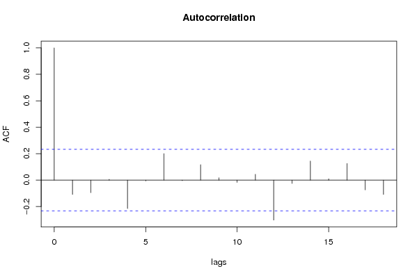
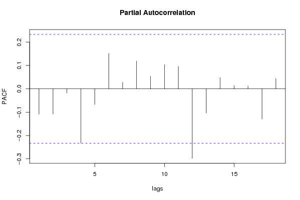
Title produced by software

(Partial) Autocorrelation Function

Date of computation

Thu, 20 Dec 2007 07:33:34 -0700

Cite this page as follows

Statistical Computations at FreeStatistics.org, Office for Research Development and Education, URL https://freestatistics.org/blog/index.php?v=date/2007/Dec/20/t11981601392hc8rqfkvjdbrs9.htm/, Retrieved Mon, 29 Apr 2024 15:40:44 +0000

Statistical Computations at FreeStatistics.org, Office for Research Development and Education, URL https://freestatistics.org/blog/index.php?pk=4722, Retrieved Mon, 29 Apr 2024 15:40:44 +0000

QR Codes:

Paste this QR Code to cite your computation.

Original text written by user:

IsPrivate?

No (this computation is public)

User-defined keywords

Estimated Impact

218

Family? (F = Feedback message, R = changed R code, M = changed R Module, P = changed Parameters, D = changed Data)

-       [(Partial) Autocorrelation Function] [infl] [2007-12-20 14:33:34] [157a0cf3c12a7482b4e6935b4c49d48f] [Current]

Feedback Forum

Post a new message

Dataseries X:

Download CSV

Histogram

Boxplots

0,3
2,1
2,5
2,3
2,4
3,0
1,7
3,5
4,0
3,7
3,7
3,0
2,7
2,5
2,2
2,9
3,1
3,0
2,8
2,5
1,9
1,9
1,8
2,0
2,6
2,5
2,5
1,6
1,4
0,8
1,1
1,3
1,2
1,3
1,1
1,3
1,2
1,6
1,7
1,5
0,9
1,5
1,4
1,6
1,7
1,4
1,8
1,7
1,4
1,2
1,0
1,7
2,4
2,0
2,1
2,0
1,8
2,7
2,3
1,9
2,0
2,3
2,8
2,4
2,3
2,7
2,7
2,9
3,0
2,2
2,3
2,8

Summary of compuational transaction
Raw Input	view raw input (R code)
Raw Output	view raw output of R engine
Computing time	3 seconds
R Server	'Herman Ole Andreas Wold' @ 193.190.124.10:1001

\begin{tabular}{lllllllll}
\hline
Summary of compuational transaction \tabularnewline
Raw Input & view raw input (R code)  \tabularnewline
Raw Output & view raw output of R engine  \tabularnewline
Computing time & 3 seconds \tabularnewline
R Server & 'Herman Ole Andreas Wold' @ 193.190.124.10:1001 \tabularnewline
\hline
\end{tabular}
%Source: https://freestatistics.org/blog/index.php?pk=4722&T=0

[TABLE]
[ROW][C]Summary of compuational transaction[/C][/ROW]
[ROW][C]Raw Input[/C][C]view raw input (R code) [/C][/ROW]
[ROW][C]Raw Output[/C][C]view raw output of R engine [/C][/ROW]
[ROW][C]Computing time[/C][C]3 seconds[/C][/ROW]
[ROW][C]R Server[/C][C]'Herman Ole Andreas Wold' @ 193.190.124.10:1001[/C][/ROW]
[/TABLE]
Source: https://freestatistics.org/blog/index.php?pk=4722&T=0

Globally Unique Identifier (entire table): ba.freestatistics.org/blog/index.php?pk=4722&T=0

As an alternative you can also use a QR Code:

The GUIDs for individual cells are displayed in the table below:

Summary of compuational transaction
Raw Input	view raw input (R code)
Raw Output	view raw output of R engine
Computing time	3 seconds
R Server	'Herman Ole Andreas Wold' @ 193.190.124.10:1001

Autocorrelation Function
Time lag k	ACF(k)	T-STAT	P-value
0	1	8.4261	0
1	-0.108903	-0.9176	0.81904
2	-0.095202	-0.8022	0.787438
3	0.005652	0.0476	0.481075
4	-0.215358	-1.8146	0.963098
5	-0.005875	-0.0495	0.51967
6	0.200053	1.6857	0.048124
7	-0.00425	-0.0358	0.514234
8	0.116585	0.9824	0.164629
9	0.017825	0.1502	0.440517
10	-0.017412	-0.1467	0.558114
11	0.04402	0.3709	0.3559
12	-0.302342	-2.5476	0.993493
13	-0.02553	-0.2151	0.584854
14	0.144313	1.216	0.114005
15	0.009461	0.0797	0.468341
16	0.126176	1.0632	0.145652
17	-0.073929	-0.6229	0.732339

\begin{tabular}{lllllllll}
\hline
Autocorrelation Function \tabularnewline
Time lag k & ACF(k) & T-STAT & P-value \tabularnewline
0 & 1 & 8.4261 & 0 \tabularnewline
1 & -0.108903 & -0.9176 & 0.81904 \tabularnewline
2 & -0.095202 & -0.8022 & 0.787438 \tabularnewline
3 & 0.005652 & 0.0476 & 0.481075 \tabularnewline
4 & -0.215358 & -1.8146 & 0.963098 \tabularnewline
5 & -0.005875 & -0.0495 & 0.51967 \tabularnewline
6 & 0.200053 & 1.6857 & 0.048124 \tabularnewline
7 & -0.00425 & -0.0358 & 0.514234 \tabularnewline
8 & 0.116585 & 0.9824 & 0.164629 \tabularnewline
9 & 0.017825 & 0.1502 & 0.440517 \tabularnewline
10 & -0.017412 & -0.1467 & 0.558114 \tabularnewline
11 & 0.04402 & 0.3709 & 0.3559 \tabularnewline
12 & -0.302342 & -2.5476 & 0.993493 \tabularnewline
13 & -0.02553 & -0.2151 & 0.584854 \tabularnewline
14 & 0.144313 & 1.216 & 0.114005 \tabularnewline
15 & 0.009461 & 0.0797 & 0.468341 \tabularnewline
16 & 0.126176 & 1.0632 & 0.145652 \tabularnewline
17 & -0.073929 & -0.6229 & 0.732339 \tabularnewline
\hline
\end{tabular}
%Source: https://freestatistics.org/blog/index.php?pk=4722&T=1

[TABLE]
[ROW][C]Autocorrelation Function[/C][/ROW]
[ROW][C]Time lag k[/C][C]ACF(k)[/C][C]T-STAT[/C][C]P-value[/C][/ROW]
[ROW][C]0[/C][C]1[/C][C]8.4261[/C][C]0[/C][/ROW]
[ROW][C]1[/C][C]-0.108903[/C][C]-0.9176[/C][C]0.81904[/C][/ROW]
[ROW][C]2[/C][C]-0.095202[/C][C]-0.8022[/C][C]0.787438[/C][/ROW]
[ROW][C]3[/C][C]0.005652[/C][C]0.0476[/C][C]0.481075[/C][/ROW]
[ROW][C]4[/C][C]-0.215358[/C][C]-1.8146[/C][C]0.963098[/C][/ROW]
[ROW][C]5[/C][C]-0.005875[/C][C]-0.0495[/C][C]0.51967[/C][/ROW]
[ROW][C]6[/C][C]0.200053[/C][C]1.6857[/C][C]0.048124[/C][/ROW]
[ROW][C]7[/C][C]-0.00425[/C][C]-0.0358[/C][C]0.514234[/C][/ROW]
[ROW][C]8[/C][C]0.116585[/C][C]0.9824[/C][C]0.164629[/C][/ROW]
[ROW][C]9[/C][C]0.017825[/C][C]0.1502[/C][C]0.440517[/C][/ROW]
[ROW][C]10[/C][C]-0.017412[/C][C]-0.1467[/C][C]0.558114[/C][/ROW]
[ROW][C]11[/C][C]0.04402[/C][C]0.3709[/C][C]0.3559[/C][/ROW]
[ROW][C]12[/C][C]-0.302342[/C][C]-2.5476[/C][C]0.993493[/C][/ROW]
[ROW][C]13[/C][C]-0.02553[/C][C]-0.2151[/C][C]0.584854[/C][/ROW]
[ROW][C]14[/C][C]0.144313[/C][C]1.216[/C][C]0.114005[/C][/ROW]
[ROW][C]15[/C][C]0.009461[/C][C]0.0797[/C][C]0.468341[/C][/ROW]
[ROW][C]16[/C][C]0.126176[/C][C]1.0632[/C][C]0.145652[/C][/ROW]
[ROW][C]17[/C][C]-0.073929[/C][C]-0.6229[/C][C]0.732339[/C][/ROW]
[/TABLE]
Source: https://freestatistics.org/blog/index.php?pk=4722&T=1

Globally Unique Identifier (entire table): ba.freestatistics.org/blog/index.php?pk=4722&T=1

As an alternative you can also use a QR Code:

The GUIDs for individual cells are displayed in the table below:

Autocorrelation Function
Time lag k	ACF(k)	T-STAT	P-value
0	1	8.4261	0
1	-0.108903	-0.9176	0.81904
2	-0.095202	-0.8022	0.787438
3	0.005652	0.0476	0.481075
4	-0.215358	-1.8146	0.963098
5	-0.005875	-0.0495	0.51967
6	0.200053	1.6857	0.048124
7	-0.00425	-0.0358	0.514234
8	0.116585	0.9824	0.164629
9	0.017825	0.1502	0.440517
10	-0.017412	-0.1467	0.558114
11	0.04402	0.3709	0.3559
12	-0.302342	-2.5476	0.993493
13	-0.02553	-0.2151	0.584854
14	0.144313	1.216	0.114005
15	0.009461	0.0797	0.468341
16	0.126176	1.0632	0.145652
17	-0.073929	-0.6229	0.732339

Partial Autocorrelation Function
Time lag k	PACF(k)	T-STAT	P-value
0	-0.108903	-0.9176	0.81904
1	-0.108347	-0.9129	0.817819
2	-0.018062	-0.1522	0.560267
3	-0.232687	-1.9607	0.973079
4	-0.067364	-0.5676	0.713959
5	0.151453	1.2762	0.103029
6	0.02762	0.2327	0.408319
7	0.119208	1.0045	0.159284
8	0.053964	0.4547	0.325354
9	0.103565	0.8727	0.192897
10	0.095998	0.8089	0.21064
11	-0.297689	-2.5084	0.992792
12	-0.104015	-0.8764	0.808128
13	0.048095	0.4053	0.343254
14	0.013685	0.1153	0.454261
15	0.012653	0.1066	0.457697
16	-0.129712	-1.093	0.860951
17	0.044198	0.3724	0.355346

\begin{tabular}{lllllllll}
\hline
Partial Autocorrelation Function \tabularnewline
Time lag k & PACF(k) & T-STAT & P-value \tabularnewline
0 & -0.108903 & -0.9176 & 0.81904 \tabularnewline
1 & -0.108347 & -0.9129 & 0.817819 \tabularnewline
2 & -0.018062 & -0.1522 & 0.560267 \tabularnewline
3 & -0.232687 & -1.9607 & 0.973079 \tabularnewline
4 & -0.067364 & -0.5676 & 0.713959 \tabularnewline
5 & 0.151453 & 1.2762 & 0.103029 \tabularnewline
6 & 0.02762 & 0.2327 & 0.408319 \tabularnewline
7 & 0.119208 & 1.0045 & 0.159284 \tabularnewline
8 & 0.053964 & 0.4547 & 0.325354 \tabularnewline
9 & 0.103565 & 0.8727 & 0.192897 \tabularnewline
10 & 0.095998 & 0.8089 & 0.21064 \tabularnewline
11 & -0.297689 & -2.5084 & 0.992792 \tabularnewline
12 & -0.104015 & -0.8764 & 0.808128 \tabularnewline
13 & 0.048095 & 0.4053 & 0.343254 \tabularnewline
14 & 0.013685 & 0.1153 & 0.454261 \tabularnewline
15 & 0.012653 & 0.1066 & 0.457697 \tabularnewline
16 & -0.129712 & -1.093 & 0.860951 \tabularnewline
17 & 0.044198 & 0.3724 & 0.355346 \tabularnewline
\hline
\end{tabular}
%Source: https://freestatistics.org/blog/index.php?pk=4722&T=2

[TABLE]
[ROW][C]Partial Autocorrelation Function[/C][/ROW]
[ROW][C]Time lag k[/C][C]PACF(k)[/C][C]T-STAT[/C][C]P-value[/C][/ROW]
[ROW][C]0[/C][C]-0.108903[/C][C]-0.9176[/C][C]0.81904[/C][/ROW]
[ROW][C]1[/C][C]-0.108347[/C][C]-0.9129[/C][C]0.817819[/C][/ROW]
[ROW][C]2[/C][C]-0.018062[/C][C]-0.1522[/C][C]0.560267[/C][/ROW]
[ROW][C]3[/C][C]-0.232687[/C][C]-1.9607[/C][C]0.973079[/C][/ROW]
[ROW][C]4[/C][C]-0.067364[/C][C]-0.5676[/C][C]0.713959[/C][/ROW]
[ROW][C]5[/C][C]0.151453[/C][C]1.2762[/C][C]0.103029[/C][/ROW]
[ROW][C]6[/C][C]0.02762[/C][C]0.2327[/C][C]0.408319[/C][/ROW]
[ROW][C]7[/C][C]0.119208[/C][C]1.0045[/C][C]0.159284[/C][/ROW]
[ROW][C]8[/C][C]0.053964[/C][C]0.4547[/C][C]0.325354[/C][/ROW]
[ROW][C]9[/C][C]0.103565[/C][C]0.8727[/C][C]0.192897[/C][/ROW]
[ROW][C]10[/C][C]0.095998[/C][C]0.8089[/C][C]0.21064[/C][/ROW]
[ROW][C]11[/C][C]-0.297689[/C][C]-2.5084[/C][C]0.992792[/C][/ROW]
[ROW][C]12[/C][C]-0.104015[/C][C]-0.8764[/C][C]0.808128[/C][/ROW]
[ROW][C]13[/C][C]0.048095[/C][C]0.4053[/C][C]0.343254[/C][/ROW]
[ROW][C]14[/C][C]0.013685[/C][C]0.1153[/C][C]0.454261[/C][/ROW]
[ROW][C]15[/C][C]0.012653[/C][C]0.1066[/C][C]0.457697[/C][/ROW]
[ROW][C]16[/C][C]-0.129712[/C][C]-1.093[/C][C]0.860951[/C][/ROW]
[ROW][C]17[/C][C]0.044198[/C][C]0.3724[/C][C]0.355346[/C][/ROW]
[/TABLE]
Source: https://freestatistics.org/blog/index.php?pk=4722&T=2

Globally Unique Identifier (entire table): ba.freestatistics.org/blog/index.php?pk=4722&T=2

As an alternative you can also use a QR Code:

The GUIDs for individual cells are displayed in the table below:

Partial Autocorrelation Function
Time lag k	PACF(k)	T-STAT	P-value
0	-0.108903	-0.9176	0.81904
1	-0.108347	-0.9129	0.817819
2	-0.018062	-0.1522	0.560267
3	-0.232687	-1.9607	0.973079
4	-0.067364	-0.5676	0.713959
5	0.151453	1.2762	0.103029
6	0.02762	0.2327	0.408319
7	0.119208	1.0045	0.159284
8	0.053964	0.4547	0.325354
9	0.103565	0.8727	0.192897
10	0.095998	0.8089	0.21064
11	-0.297689	-2.5084	0.992792
12	-0.104015	-0.8764	0.808128
13	0.048095	0.4053	0.343254
14	0.013685	0.1153	0.454261
15	0.012653	0.1066	0.457697
16	-0.129712	-1.093	0.860951
17	0.044198	0.3724	0.355346

Figure 1

PNG link

Postscript link

PDF link

Figure 2

PNG link

Postscript link

PDF link

Parameters (Session):

par1 = Default ; par2 = 1 ; par3 = 1 ; par4 = 0 ; par5 = 12 ;

Parameters (R input):

par1 = Default ; par2 = 1 ; par3 = 1 ; par4 = 0 ; par5 = 12 ;

R code (references can be found in the software module):

if (par1 == 'Default') {
par1 = 10*log10(length(x))
} else {
par1 <- as.numeric(par1)
}
par2 <- as.numeric(par2)
par3 <- as.numeric(par3)
par4 <- as.numeric(par4)
par5 <- as.numeric(par5)
if (par2 == 0) {
x <- log(x)
} else {
x <- (x ^ par2 - 1) / par2
}
if (par3 > 0) x <- diff(x,lag=1,difference=par3)
if (par4 > 0) x <- diff(x,lag=par5,difference=par4)
bitmap(file='pic1.png')
racf <- acf(x,par1,main='Autocorrelation',xlab='lags',ylab='ACF')
dev.off()
bitmap(file='pic2.png')
rpacf <- pacf(x,par1,main='Partial Autocorrelation',xlab='lags',ylab='PACF')
dev.off()
(myacf <- c(racf$acf))
(mypacf <- c(rpacf$acf))
lengthx <- length(x)
sqrtn <- sqrt(lengthx)
load(file='createtable')
a<-table.start()
a<-table.row.start(a)
a<-table.element(a,'Autocorrelation Function',4,TRUE)
a<-table.row.end(a)
a<-table.row.start(a)
a<-table.element(a,'Time lag k',header=TRUE)
a<-table.element(a,hyperlink('basics.htm','ACF(k)','click here for more information about the Autocorrelation Function'),header=TRUE)
a<-table.element(a,'T-STAT',header=TRUE)
a<-table.element(a,'P-value',header=TRUE)
a<-table.row.end(a)
for (i in 1:par1) {
a<-table.row.start(a)
a<-table.element(a,i-1,header=TRUE)
a<-table.element(a,round(myacf[i],6))
mytstat <- myacf[i]*sqrtn
a<-table.element(a,round(mytstat,4))
a<-table.element(a,round(1-pt(mytstat,lengthx),6))
a<-table.row.end(a)
}
a<-table.end(a)
table.save(a,file='mytable.tab')
a<-table.start()
a<-table.row.start(a)
a<-table.element(a,'Partial Autocorrelation Function',4,TRUE)
a<-table.row.end(a)
a<-table.row.start(a)
a<-table.element(a,'Time lag k',header=TRUE)
a<-table.element(a,hyperlink('basics.htm','PACF(k)','click here for more information about the Partial Autocorrelation Function'),header=TRUE)
a<-table.element(a,'T-STAT',header=TRUE)
a<-table.element(a,'P-value',header=TRUE)
a<-table.row.end(a)
for (i in 1:par1) {
a<-table.row.start(a)
a<-table.element(a,i-1,header=TRUE)
a<-table.element(a,round(mypacf[i],6))
mytstat <- mypacf[i]*sqrtn
a<-table.element(a,round(mytstat,4))
a<-table.element(a,round(1-pt(mytstat,lengthx),6))
a<-table.row.end(a)
}
a<-table.end(a)
table.save(a,file='mytable1.tab')

Free Statistics

Description of Statistical Computation

Tree of Dependent Computations

Dataset

Tables (Output of Computation)

Figures (Output of Computation)

Input Parameters & R Code