Free Statistics
of Irreproducible Research!
Description of Statistical Computation | |||||||||||||||||||||||||||||||||||||||||||||||||||||
|---|---|---|---|---|---|---|---|---|---|---|---|---|---|---|---|---|---|---|---|---|---|---|---|---|---|---|---|---|---|---|---|---|---|---|---|---|---|---|---|---|---|---|---|---|---|---|---|---|---|---|---|---|---|
| Author's title | |||||||||||||||||||||||||||||||||||||||||||||||||||||
| Author | *Unverified author* | ||||||||||||||||||||||||||||||||||||||||||||||||||||
| R Software Module | rwasp_edauni.wasp | ||||||||||||||||||||||||||||||||||||||||||||||||||||
| Title produced by software | Univariate Explorative Data Analysis | ||||||||||||||||||||||||||||||||||||||||||||||||||||
| Date of computation | Tue, 18 Dec 2007 14:10:49 -0700 | ||||||||||||||||||||||||||||||||||||||||||||||||||||
| Cite this page as follows | Statistical Computations at FreeStatistics.org, Office for Research Development and Education, URL https://freestatistics.org/blog/index.php?v=date/2007/Dec/18/t1198011229h93f5ncuoibmzf8.htm/, Retrieved Tue, 15 Jul 2025 19:29:39 +0000 | ||||||||||||||||||||||||||||||||||||||||||||||||||||
| Statistical Computations at FreeStatistics.org, Office for Research Development and Education, URL https://freestatistics.org/blog/index.php?pk=4614, Retrieved Tue, 15 Jul 2025 19:29:39 +0000 | |||||||||||||||||||||||||||||||||||||||||||||||||||||
| QR Codes: | |||||||||||||||||||||||||||||||||||||||||||||||||||||
|
| |||||||||||||||||||||||||||||||||||||||||||||||||||||
| Original text written by user: | |||||||||||||||||||||||||||||||||||||||||||||||||||||
| IsPrivate? | No (this computation is public) | ||||||||||||||||||||||||||||||||||||||||||||||||||||
| User-defined keywords | PUEDARM | ||||||||||||||||||||||||||||||||||||||||||||||||||||
| Estimated Impact | 357 | ||||||||||||||||||||||||||||||||||||||||||||||||||||
Tree of Dependent Computations | |||||||||||||||||||||||||||||||||||||||||||||||||||||
| Family? (F = Feedback message, R = changed R code, M = changed R Module, P = changed Parameters, D = changed Data) | |||||||||||||||||||||||||||||||||||||||||||||||||||||
| - [Univariate Explorative Data Analysis] [Paper - Univerate...] [2007-12-18 21:10:49] [e51d7ab0e549b3dc96ac85a81d9bd259] [Current] - D [Univariate Explorative Data Analysis] [Paper - Univerate...] [2008-12-28 14:26:36] [c29178f7f550574a75dc881e636e0923] - D [Univariate Explorative Data Analysis] [Paper - Univerate...] [2008-12-28 14:30:01] [c29178f7f550574a75dc881e636e0923] - D [Univariate Explorative Data Analysis] [http://www.freest...] [2008-12-28 14:36:31] [c29178f7f550574a75dc881e636e0923] | |||||||||||||||||||||||||||||||||||||||||||||||||||||
| Feedback Forum | |||||||||||||||||||||||||||||||||||||||||||||||||||||
Post a new message | |||||||||||||||||||||||||||||||||||||||||||||||||||||
Dataset | |||||||||||||||||||||||||||||||||||||||||||||||||||||
| Dataseries X: | |||||||||||||||||||||||||||||||||||||||||||||||||||||
2.61072861587664 -1.64151512748939 -5.53397130675664 -11.8684507675144 4.92307208512571 6.26712823161773 -2.76872599233773 -3.56312607919330 3.84610531691476 3.92414528449639 -2.60085355983359 -4.52415672464345 0.712363410392165 -3.83027221556495 1.64369314986718 5.1373157082981 -4.77891279135298 -0.543348509239105 10.7317442356705 -7.66239213978311 -6.30680235597392 -7.34729981849825 0.617800822224108 2.85035364935883 1.77740032934145 -3.90118201853709 4.6323076169406 -1.74030963922678 -3.27944132766354 1.09665938498306 7.05463838922537 2.50775091630909 -4.16477564673257 -3.97156359496111 -4.61876313016936 -1.80864980481552 -0.236907168104795 -3.15041173459177 3.37110805438328 -2.30793345402054 2.737897737493 -1.58208769004317 -2.47767476900079 0.167763916859109 1.76974633325578 0.440544884754961 -2.45008188331654 4.47063460393658 -6.94943202424074 8.91682112964061 -0.296516314946182 2.40580572796091 -1.75212202583747 5.39306701500983 6.30609401440519 7.82784320522538 -2.60554495964265 1.29269020570918 1.09083902934299 0.640809564220057 -0.654553416503333 3.45822878067978 1.27021269162882 -1.88415061828193 0.908614567669563 | |||||||||||||||||||||||||||||||||||||||||||||||||||||
Tables (Output of Computation) | |||||||||||||||||||||||||||||||||||||||||||||||||||||
| |||||||||||||||||||||||||||||||||||||||||||||||||||||
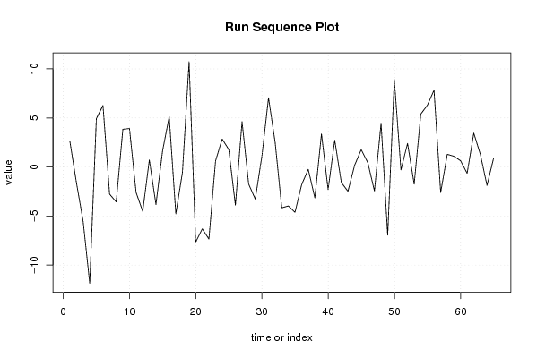
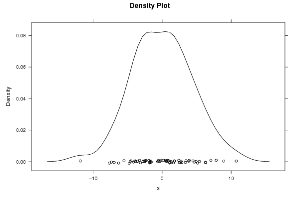
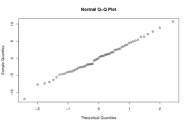
Figures (Output of Computation) | |||||||||||||||||||||||||||||||||||||||||||||||||||||
Input Parameters & R Code | |||||||||||||||||||||||||||||||||||||||||||||||||||||
| Parameters (Session): | |||||||||||||||||||||||||||||||||||||||||||||||||||||
| par1 = 0 ; par2 = 36 ; | |||||||||||||||||||||||||||||||||||||||||||||||||||||
| Parameters (R input): | |||||||||||||||||||||||||||||||||||||||||||||||||||||
| par1 = 0 ; par2 = 36 ; | |||||||||||||||||||||||||||||||||||||||||||||||||||||
| R code (references can be found in the software module): | |||||||||||||||||||||||||||||||||||||||||||||||||||||
par1 <- as.numeric(par1) | |||||||||||||||||||||||||||||||||||||||||||||||||||||