Repository of Reproducible Computations

Free Statistics

of Irreproducible Research!

Author's title

Author

*Unverified author*

R Software Module

rwasp_edauni.wasp

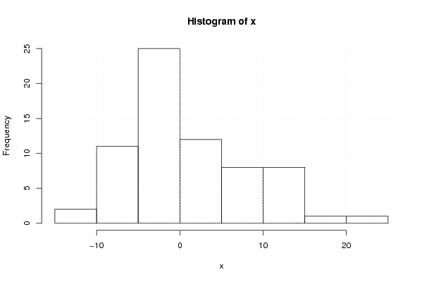
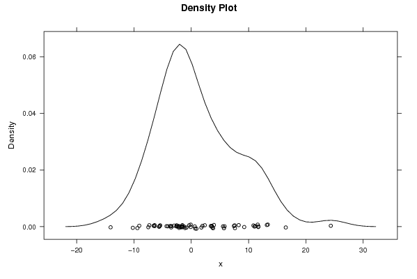
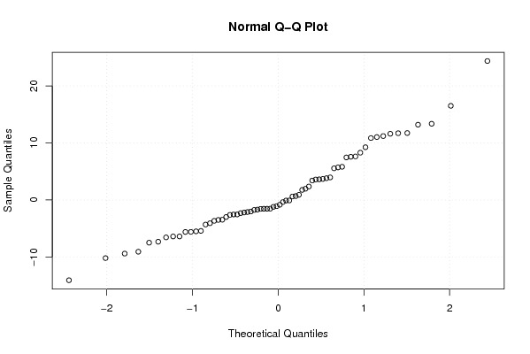
Title produced by software

Univariate Explorative Data Analysis

Date of computation

Tue, 18 Dec 2007 07:03:15 -0700

Cite this page as follows

Statistical Computations at FreeStatistics.org, Office for Research Development and Education, URL https://freestatistics.org/blog/index.php?v=date/2007/Dec/18/t1197985572pe57klecn2pxntv.htm/, Retrieved Sat, 04 May 2024 19:10:08 +0000

Statistical Computations at FreeStatistics.org, Office for Research Development and Education, URL https://freestatistics.org/blog/index.php?pk=4517, Retrieved Sat, 04 May 2024 19:10:08 +0000

QR Codes:

Paste this QR Code to cite your computation.

Original text written by user:

IsPrivate?

No (this computation is public)

User-defined keywords

Estimated Impact

230

Family? (F = Feedback message, R = changed R code, M = changed R Module, P = changed Parameters, D = changed Data)

-       [Univariate Explorative Data Analysis] [Paper-univariate ...] [2007-12-18 14:03:15] [5b9249e3962a4d9b95a2c513d8084bf7] [Current]
-   PD    [Univariate Explorative Data Analysis] [Paper-univariate ...] [2008-12-27 12:26:50] [1aad2bd7746abaf3ab17fe0d80878872] 
-   PD    [Univariate Explorative Data Analysis] [Paper-univariate ...] [2008-12-27 12:30:35] [1aad2bd7746abaf3ab17fe0d80878872] 
-   PD    [Univariate Explorative Data Analysis] [Paper-univariate ...] [2008-12-27 12:35:23] [1aad2bd7746abaf3ab17fe0d80878872] 

Feedback Forum

Post a new message

Dataseries X:

Download CSV

Histogram

Boxplots

-0.361846007532772 
3.68863098861213 
0.682519663180303 
7.63067731671178 
-1.52075037210644 
5.70955581144987 
13.1939928862509 
-5.49940323517293 
1.76500444649349 
1.96677142422135 
-5.60662922820024 
-7.31646013152379 
-1.08563548801227 
-0.099103421317697 
-9.39514313732207 
-6.39447775845358 
-2.02805473224696 
0.903602088633067 
7.57491469457003 
-2.19407311445752 
3.58898833702079 
-1.68951274457543 
-1.53671157669086 
13.3598886375142 
-3.65726657887787 
0.613493186862468 
9.24506908223031 
11.0285738876639 
-3.49893748343257 
-6.55850163797107 
5.54750744110568 
16.5005808635365 
-0.0867999869147866 
-10.1895526735612 
-1.56002146200367 
3.61791774409454 
-3.46228026897451 
-0.839719033549138 
-1.74844063591575 
-5.59275453302008 
-4.31083509741400 
8.28778989827125 
-14.0676602788114 
-4.07578881412959 
3.95794121224257 
-2.54404876219145 
24.3555160491049 
11.7342693021934 
3.81944484749606 
-2.98176766619709 
7.45551605729516 
-6.39245158356992 
11.7003155629076 
2.36027611470617 
-7.48442696186156 
-2.54111530629837 
-2.30507409276129 
10.8550201878513 
-2.11331989623902 
3.4086895867965 
11.2003605872847 
-1.20537867882487 
5.81786820725412 
-2.61150202837964 
-1.54008349441135 
-5.42145151519334 
11.6034074049369 
-9.06789177079852

Summary of compuational transaction
Raw Input	view raw input (R code)
Raw Output	view raw output of R engine
Computing time	3 seconds
R Server	'Gwilym Jenkins' @ 72.249.127.135

\begin{tabular}{lllllllll}
\hline
Summary of compuational transaction \tabularnewline
Raw Input & view raw input (R code)  \tabularnewline
Raw Output & view raw output of R engine  \tabularnewline
Computing time & 3 seconds \tabularnewline
R Server & 'Gwilym Jenkins' @ 72.249.127.135 \tabularnewline
\hline
\end{tabular}
%Source: https://freestatistics.org/blog/index.php?pk=4517&T=0

[TABLE]
[ROW][C]Summary of compuational transaction[/C][/ROW]
[ROW][C]Raw Input[/C][C]view raw input (R code) [/C][/ROW]
[ROW][C]Raw Output[/C][C]view raw output of R engine [/C][/ROW]
[ROW][C]Computing time[/C][C]3 seconds[/C][/ROW]
[ROW][C]R Server[/C][C]'Gwilym Jenkins' @ 72.249.127.135[/C][/ROW]
[/TABLE]
Source: https://freestatistics.org/blog/index.php?pk=4517&T=0

Globally Unique Identifier (entire table): ba.freestatistics.org/blog/index.php?pk=4517&T=0

As an alternative you can also use a QR Code:

The GUIDs for individual cells are displayed in the table below:

Summary of compuational transaction
Raw Input	view raw input (R code)
Raw Output	view raw output of R engine
Computing time	3 seconds
R Server	'Gwilym Jenkins' @ 72.249.127.135

Descriptive Statistics
# observations	68
minimum	-14.0676602788114
Q1	-3.47144457258903
median	-0.962677260780704
mean	1.06748871072908
Q3	5.58801953369173
maximum	24.3555160491049

\begin{tabular}{lllllllll}
\hline
Descriptive Statistics \tabularnewline
# observations & 68 \tabularnewline
minimum & -14.0676602788114 \tabularnewline
Q1 & -3.47144457258903 \tabularnewline
median & -0.962677260780704 \tabularnewline
mean & 1.06748871072908 \tabularnewline
Q3 & 5.58801953369173 \tabularnewline
maximum & 24.3555160491049 \tabularnewline
\hline
\end{tabular}
%Source: https://freestatistics.org/blog/index.php?pk=4517&T=1

[TABLE]
[ROW][C]Descriptive Statistics[/C][/ROW]
[ROW][C]# observations[/C][C]68[/C][/ROW]
[ROW][C]minimum[/C][C]-14.0676602788114[/C][/ROW]
[ROW][C]Q1[/C][C]-3.47144457258903[/C][/ROW]
[ROW][C]median[/C][C]-0.962677260780704[/C][/ROW]
[ROW][C]mean[/C][C]1.06748871072908[/C][/ROW]
[ROW][C]Q3[/C][C]5.58801953369173[/C][/ROW]
[ROW][C]maximum[/C][C]24.3555160491049[/C][/ROW]
[/TABLE]
Source: https://freestatistics.org/blog/index.php?pk=4517&T=1

Globally Unique Identifier (entire table): ba.freestatistics.org/blog/index.php?pk=4517&T=1

As an alternative you can also use a QR Code:

The GUIDs for individual cells are displayed in the table below:

Descriptive Statistics
# observations	68
minimum	-14.0676602788114
Q1	-3.47144457258903
median	-0.962677260780704
mean	1.06748871072908
Q3	5.58801953369173
maximum	24.3555160491049

Figure 1

PNG link

Postscript link

PDF link

Figure 2

PNG link

Postscript link

PDF link

Figure 3

PNG link

Postscript link

PDF link

Figure 4

PNG link

Postscript link

PDF link

Figure 5

PNG link

Postscript link

PDF link

Figure 6

PNG link

Postscript link

PDF link

Parameters (Session):

par1 = 0 ; par2 = 30 ;

Parameters (R input):

par1 = 0 ; par2 = 30 ;

R code (references can be found in the software module):

par1 <- as.numeric(par1)
par2 <- as.numeric(par2)
x <- as.ts(x)
library(lattice)
bitmap(file='pic1.png')
plot(x,type='l',main='Run Sequence Plot',xlab='time or index',ylab='value')
grid()
dev.off()
bitmap(file='pic2.png')
hist(x)
grid()
dev.off()
bitmap(file='pic3.png')
if (par1 > 0)
{
densityplot(~x,col='black',main=paste('Density Plot   bw = ',par1),bw=par1)
} else {
densityplot(~x,col='black',main='Density Plot')
}
dev.off()
bitmap(file='pic4.png')
qqnorm(x)
grid()
dev.off()
if (par2 > 0)
{
bitmap(file='lagplot.png')
dum <- cbind(lag(x,k=1),x)
dum
dum1 <- dum[2:length(x),]
dum1
z <- as.data.frame(dum1)
z
plot(z,main=paste('Lag plot, lowess, and regression line'))
lines(lowess(z))
abline(lm(z))
dev.off()
bitmap(file='pic5.png')
acf(x,lag.max=par2,main='Autocorrelation Function')
grid()
dev.off()
}
summary(x)
load(file='createtable')
a<-table.start()
a<-table.row.start(a)
a<-table.element(a,'Descriptive Statistics',2,TRUE)
a<-table.row.end(a)
a<-table.row.start(a)
a<-table.element(a,'# observations',header=TRUE)
a<-table.element(a,length(x))
a<-table.row.end(a)
a<-table.row.start(a)
a<-table.element(a,'minimum',header=TRUE)
a<-table.element(a,min(x))
a<-table.row.end(a)
a<-table.row.start(a)
a<-table.element(a,'Q1',header=TRUE)
a<-table.element(a,quantile(x,0.25))
a<-table.row.end(a)
a<-table.row.start(a)
a<-table.element(a,'median',header=TRUE)
a<-table.element(a,median(x))
a<-table.row.end(a)
a<-table.row.start(a)
a<-table.element(a,'mean',header=TRUE)
a<-table.element(a,mean(x))
a<-table.row.end(a)
a<-table.row.start(a)
a<-table.element(a,'Q3',header=TRUE)
a<-table.element(a,quantile(x,0.75))
a<-table.row.end(a)
a<-table.row.start(a)
a<-table.element(a,'maximum',header=TRUE)
a<-table.element(a,max(x))
a<-table.row.end(a)
a<-table.end(a)
table.save(a,file='mytable.tab')

Free Statistics

Description of Statistical Computation

Tree of Dependent Computations

Dataset

Tables (Output of Computation)

Figures (Output of Computation)

Input Parameters & R Code