Repository of Reproducible Computations

Free Statistics

of Irreproducible Research!

Author's title

Author

*Unverified author*

R Software Module

rwasp_edauni.wasp

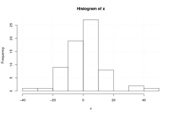
Title produced by software

Univariate Explorative Data Analysis

Date of computation

Mon, 17 Dec 2007 12:35:28 -0700

Cite this page as follows

Statistical Computations at FreeStatistics.org, Office for Research Development and Education, URL https://freestatistics.org/blog/index.php?v=date/2007/Dec/17/t1197919133jun07ja3a2z5sdu.htm/, Retrieved Fri, 03 May 2024 20:18:48 +0000

Statistical Computations at FreeStatistics.org, Office for Research Development and Education, URL https://freestatistics.org/blog/index.php?pk=4416, Retrieved Fri, 03 May 2024 20:18:48 +0000

QR Codes:

Paste this QR Code to cite your computation.

Original text written by user:

IsPrivate?

No (this computation is public)

User-defined keywords

P4PRMA

Estimated Impact

204

Family? (F = Feedback message, R = changed R code, M = changed R Module, P = changed Parameters, D = changed Data)

-       [Univariate Explorative Data Analysis] [Paper - 4plot - R...] [2007-12-17 19:35:28] [e51d7ab0e549b3dc96ac85a81d9bd259] [Current]
-   PD    [Univariate Explorative Data Analysis] [Paper - 4plot - R...] [2008-12-27 13:10:15] [1aad2bd7746abaf3ab17fe0d80878872] 
-   PD    [Univariate Explorative Data Analysis] [Paper - 4plot - R...] [2008-12-27 13:11:29] [1aad2bd7746abaf3ab17fe0d80878872] 
-   PD    [Univariate Explorative Data Analysis] [Paper - 4plot - R...] [2008-12-27 13:16:03] [1aad2bd7746abaf3ab17fe0d80878872] 

Feedback Forum

Post a new message

Dataseries X:

Download CSV

Histogram

Boxplots

-0.385868851153837
4.81234262686034
-5.86804122114596
16.0725680225492
-8.57525163788969
5.08247518971098
0.092732021505415
3.83298655010795
5.81986266263392
37.1247698411582
-0.456916305824569
-3.62813490741323
-3.87648507892191
4.61958462101272
-12.967748044016
3.19886759717217
-5.74783565702396
-0.568909646003526
-7.15658094463292
-18.0497313555278
15.6314099338156
-18.6819481453537
-0.704909311621681
2.59171945848611
2.56763423323193
0.363060127151921
32.5587282582796
8.52568321864334
1.42269516052334
3.53469472344553
0.904411865388995
-1.1005444418027
13.3248076718110
-33.5907843348750
-0.845486516554237
42.0892768528428
-6.25360506437205
-11.0785340316643
-29.2902232669615
-11.1727173982373
13.9239510644368
13.5369579913798
-16.4941540115674
-9.38355957013267
-2.83541693438183
-2.88173330956316
6.18397479401454
3.71189006095175
3.17508248559435
-4.18249526402528
13.6042900329871
4.81933405297545
10.0482983006261
9.69015652302726
-13.6259654676286
2.81390485024080
2.39082408194279
9.1175078099302
14.2141474796521
3.49385172983141
5.51425675339953
-6.1504957612917
2.72297593670155
-11.1163190852539
-4.69675096946234
1.81576665288666
-10.4353591925503
6.036622781552

Summary of compuational transaction
Raw Input	view raw input (R code)
Raw Output	view raw output of R engine
Computing time	2 seconds
R Server	'Gwilym Jenkins' @ 72.249.127.135

\begin{tabular}{lllllllll}
\hline
Summary of compuational transaction \tabularnewline
Raw Input & view raw input (R code)  \tabularnewline
Raw Output & view raw output of R engine  \tabularnewline
Computing time & 2 seconds \tabularnewline
R Server & 'Gwilym Jenkins' @ 72.249.127.135 \tabularnewline
\hline
\end{tabular}
%Source: https://freestatistics.org/blog/index.php?pk=4416&T=0

[TABLE]
[ROW][C]Summary of compuational transaction[/C][/ROW]
[ROW][C]Raw Input[/C][C]view raw input (R code) [/C][/ROW]
[ROW][C]Raw Output[/C][C]view raw output of R engine [/C][/ROW]
[ROW][C]Computing time[/C][C]2 seconds[/C][/ROW]
[ROW][C]R Server[/C][C]'Gwilym Jenkins' @ 72.249.127.135[/C][/ROW]
[/TABLE]
Source: https://freestatistics.org/blog/index.php?pk=4416&T=0

Globally Unique Identifier (entire table): ba.freestatistics.org/blog/index.php?pk=4416&T=0

As an alternative you can also use a QR Code:

The GUIDs for individual cells are displayed in the table below:

Summary of compuational transaction
Raw Input	view raw input (R code)
Raw Output	view raw output of R engine
Computing time	2 seconds
R Server	'Gwilym Jenkins' @ 72.249.127.135

Descriptive Statistics
# observations	68
minimum	-33.590784334875
Q1	-5.77788704805446
median	1.619230906705
mean	1.01737644546483
Q3	5.59065823070813
maximum	42.0892768528428

\begin{tabular}{lllllllll}
\hline
Descriptive Statistics \tabularnewline
# observations & 68 \tabularnewline
minimum & -33.590784334875 \tabularnewline
Q1 & -5.77788704805446 \tabularnewline
median & 1.619230906705 \tabularnewline
mean & 1.01737644546483 \tabularnewline
Q3 & 5.59065823070813 \tabularnewline
maximum & 42.0892768528428 \tabularnewline
\hline
\end{tabular}
%Source: https://freestatistics.org/blog/index.php?pk=4416&T=1

[TABLE]
[ROW][C]Descriptive Statistics[/C][/ROW]
[ROW][C]# observations[/C][C]68[/C][/ROW]
[ROW][C]minimum[/C][C]-33.590784334875[/C][/ROW]
[ROW][C]Q1[/C][C]-5.77788704805446[/C][/ROW]
[ROW][C]median[/C][C]1.619230906705[/C][/ROW]
[ROW][C]mean[/C][C]1.01737644546483[/C][/ROW]
[ROW][C]Q3[/C][C]5.59065823070813[/C][/ROW]
[ROW][C]maximum[/C][C]42.0892768528428[/C][/ROW]
[/TABLE]
Source: https://freestatistics.org/blog/index.php?pk=4416&T=1

Globally Unique Identifier (entire table): ba.freestatistics.org/blog/index.php?pk=4416&T=1

As an alternative you can also use a QR Code:

The GUIDs for individual cells are displayed in the table below:

Descriptive Statistics
# observations	68
minimum	-33.590784334875
Q1	-5.77788704805446
median	1.619230906705
mean	1.01737644546483
Q3	5.59065823070813
maximum	42.0892768528428

Figure 1

PNG link

Postscript link

PDF link

Figure 2

PNG link

Postscript link

PDF link

Figure 3

PNG link

Postscript link

PDF link

Figure 4

PNG link

Postscript link

PDF link

Figure 5

PNG link

Postscript link

PDF link

Figure 6

PNG link

Postscript link

PDF link

Parameters (Session):

par1 = 0 ; par2 = 30 ;

Parameters (R input):

par1 = 0 ; par2 = 30 ;

R code (references can be found in the software module):

par1 <- as.numeric(par1)
par2 <- as.numeric(par2)
x <- as.ts(x)
library(lattice)
bitmap(file='pic1.png')
plot(x,type='l',main='Run Sequence Plot',xlab='time or index',ylab='value')
grid()
dev.off()
bitmap(file='pic2.png')
hist(x)
grid()
dev.off()
bitmap(file='pic3.png')
if (par1 > 0)
{
densityplot(~x,col='black',main=paste('Density Plot   bw = ',par1),bw=par1)
} else {
densityplot(~x,col='black',main='Density Plot')
}
dev.off()
bitmap(file='pic4.png')
qqnorm(x)
grid()
dev.off()
if (par2 > 0)
{
bitmap(file='lagplot.png')
dum <- cbind(lag(x,k=1),x)
dum
dum1 <- dum[2:length(x),]
dum1
z <- as.data.frame(dum1)
z
plot(z,main=paste('Lag plot, lowess, and regression line'))
lines(lowess(z))
abline(lm(z))
dev.off()
bitmap(file='pic5.png')
acf(x,lag.max=par2,main='Autocorrelation Function')
grid()
dev.off()
}
summary(x)
load(file='createtable')
a<-table.start()
a<-table.row.start(a)
a<-table.element(a,'Descriptive Statistics',2,TRUE)
a<-table.row.end(a)
a<-table.row.start(a)
a<-table.element(a,'# observations',header=TRUE)
a<-table.element(a,length(x))
a<-table.row.end(a)
a<-table.row.start(a)
a<-table.element(a,'minimum',header=TRUE)
a<-table.element(a,min(x))
a<-table.row.end(a)
a<-table.row.start(a)
a<-table.element(a,'Q1',header=TRUE)
a<-table.element(a,quantile(x,0.25))
a<-table.row.end(a)
a<-table.row.start(a)
a<-table.element(a,'median',header=TRUE)
a<-table.element(a,median(x))
a<-table.row.end(a)
a<-table.row.start(a)
a<-table.element(a,'mean',header=TRUE)
a<-table.element(a,mean(x))
a<-table.row.end(a)
a<-table.row.start(a)
a<-table.element(a,'Q3',header=TRUE)
a<-table.element(a,quantile(x,0.75))
a<-table.row.end(a)
a<-table.row.start(a)
a<-table.element(a,'maximum',header=TRUE)
a<-table.element(a,max(x))
a<-table.row.end(a)
a<-table.end(a)
table.save(a,file='mytable.tab')

Free Statistics

Description of Statistical Computation

Tree of Dependent Computations

Dataset

Tables (Output of Computation)

Figures (Output of Computation)

Input Parameters & R Code