Free Statistics
of Irreproducible Research!
Description of Statistical Computation | |||||||||||||||||||||||||||||||||||||||||||||
|---|---|---|---|---|---|---|---|---|---|---|---|---|---|---|---|---|---|---|---|---|---|---|---|---|---|---|---|---|---|---|---|---|---|---|---|---|---|---|---|---|---|---|---|---|---|
| Author's title | |||||||||||||||||||||||||||||||||||||||||||||
| Author | *Unverified author* | ||||||||||||||||||||||||||||||||||||||||||||
| R Software Module | rwasp_boxcoxlin.wasp | ||||||||||||||||||||||||||||||||||||||||||||
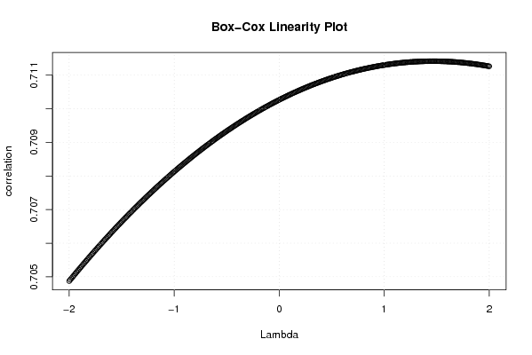
| Title produced by software | Box-Cox Linearity Plot | ||||||||||||||||||||||||||||||||||||||||||||
| Date of computation | Sun, 16 Dec 2007 03:37:52 -0700 | ||||||||||||||||||||||||||||||||||||||||||||
| Cite this page as follows | Statistical Computations at FreeStatistics.org, Office for Research Development and Education, URL https://freestatistics.org/blog/index.php?v=date/2007/Dec/16/t1197800505vc6crxfjmga204z.htm/, Retrieved Fri, 11 Jul 2025 21:00:08 +0000 | ||||||||||||||||||||||||||||||||||||||||||||
| Statistical Computations at FreeStatistics.org, Office for Research Development and Education, URL https://freestatistics.org/blog/index.php?pk=4124, Retrieved Fri, 11 Jul 2025 21:00:08 +0000 | |||||||||||||||||||||||||||||||||||||||||||||
| QR Codes: | |||||||||||||||||||||||||||||||||||||||||||||
|
| |||||||||||||||||||||||||||||||||||||||||||||
| Original text written by user: | |||||||||||||||||||||||||||||||||||||||||||||
| IsPrivate? | No (this computation is public) | ||||||||||||||||||||||||||||||||||||||||||||
| User-defined keywords | Tukey Intermediaire en Investerings | ||||||||||||||||||||||||||||||||||||||||||||
| Estimated Impact | 332 | ||||||||||||||||||||||||||||||||||||||||||||
Tree of Dependent Computations | |||||||||||||||||||||||||||||||||||||||||||||
| Family? (F = Feedback message, R = changed R code, M = changed R Module, P = changed Parameters, D = changed Data) | |||||||||||||||||||||||||||||||||||||||||||||
| - [Box-Cox Linearity Plot] [Tukey Intermediai...] [2007-12-16 10:37:52] [0cecb02636bfe8ebd97a7fef80b2b9e7] [Current] | |||||||||||||||||||||||||||||||||||||||||||||
| Feedback Forum | |||||||||||||||||||||||||||||||||||||||||||||
Post a new message | |||||||||||||||||||||||||||||||||||||||||||||
Dataset | |||||||||||||||||||||||||||||||||||||||||||||
| Dataseries X: | |||||||||||||||||||||||||||||||||||||||||||||
106,9 107,1 99,3 99,2 108,3 105,6 99,5 107,4 93,1 88,1 110,7 113,1 99,6 93,6 98,6 99,6 114,3 107,8 101,2 112,5 100,5 93,9 116,2 112,0 106,4 95,7 96,0 95,8 103,0 102,2 98,4 111,4 86,6 91,3 107,9 101,8 104,4 93,4 100,1 98,5 112,9 101,4 107,1 110,8 90,3 95,5 111,4 113,0 107,5 95,9 106,3 105,2 117,2 106,9 108,2 113,0 97,2 100,2 109,7 119,1 | |||||||||||||||||||||||||||||||||||||||||||||
| Dataseries Y: | |||||||||||||||||||||||||||||||||||||||||||||
93,9 89,8 93,4 101,5 110,4 105,9 108,4 113,9 86,1 69,4 101,2 100,5 98,0 106,6 90,1 96,9 125,9 112,0 100,0 123,9 79,8 83,4 113,6 112,9 104,0 109,9 99,0 106,3 128,9 111,1 102,9 130,0 87,0 87,5 117,6 103,4 110,8 112,6 102,5 112,4 135,6 105,1 127,7 137,0 91,0 90,5 122,4 123,3 124,3 120,0 118,1 119,0 142,7 123,6 129,6 151,6 110,4 99,3 129,1 134,1 | |||||||||||||||||||||||||||||||||||||||||||||
Tables (Output of Computation) | |||||||||||||||||||||||||||||||||||||||||||||
| |||||||||||||||||||||||||||||||||||||||||||||
Figures (Output of Computation) | |||||||||||||||||||||||||||||||||||||||||||||
Input Parameters & R Code | |||||||||||||||||||||||||||||||||||||||||||||
| Parameters (Session): | |||||||||||||||||||||||||||||||||||||||||||||
| Parameters (R input): | |||||||||||||||||||||||||||||||||||||||||||||
| R code (references can be found in the software module): | |||||||||||||||||||||||||||||||||||||||||||||
n <- length(x) | |||||||||||||||||||||||||||||||||||||||||||||