Free Statistics
of Irreproducible Research!
Description of Statistical Computation | |||||||||||||||||||||
|---|---|---|---|---|---|---|---|---|---|---|---|---|---|---|---|---|---|---|---|---|---|
| Author's title | |||||||||||||||||||||
| Author | *Unverified author* | ||||||||||||||||||||
| R Software Module | rwasp_meanplot.wasp | ||||||||||||||||||||
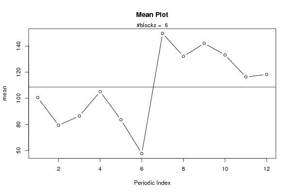
| Title produced by software | Mean Plot | ||||||||||||||||||||
| Date of computation | Sat, 15 Dec 2007 12:02:09 -0700 | ||||||||||||||||||||
| Cite this page as follows | Statistical Computations at FreeStatistics.org, Office for Research Development and Education, URL https://freestatistics.org/blog/index.php?v=date/2007/Dec/15/t1197744362iqhm2ns8uyq0wvg.htm/, Retrieved Thu, 02 May 2024 19:21:27 +0000 | ||||||||||||||||||||
| Statistical Computations at FreeStatistics.org, Office for Research Development and Education, URL https://freestatistics.org/blog/index.php?pk=4091, Retrieved Thu, 02 May 2024 19:21:27 +0000 | |||||||||||||||||||||
| QR Codes: | |||||||||||||||||||||
|
| |||||||||||||||||||||
| Original text written by user: | |||||||||||||||||||||
| IsPrivate? | No (this computation is public) | ||||||||||||||||||||
| User-defined keywords | |||||||||||||||||||||
| Estimated Impact | 195 | ||||||||||||||||||||
Tree of Dependent Computations | |||||||||||||||||||||
| Family? (F = Feedback message, R = changed R code, M = changed R Module, P = changed Parameters, D = changed Data) | |||||||||||||||||||||
| - [Mean Plot] [] [2007-12-15 19:02:09] [ba3202e2798d2e4685d19d988e9c69df] [Current] | |||||||||||||||||||||
| Feedback Forum | |||||||||||||||||||||
Post a new message | |||||||||||||||||||||
Dataset | |||||||||||||||||||||
| Dataseries X: | |||||||||||||||||||||
92,81 59,04 72,81 91,81 68,07 49,16 124,61 109,89 110,51 114,77 92,37 103,63 90,43 65,86 83,33 94,49 68,98 55,46 132,89 121,71 127,01 134,04 106,48 117,55 101,61 82,66 89,28 109,24 88,16 59,23 164,21 125,13 152,68 132,96 112,42 136,43 107,32 87,61 97,86 106,60 92,17 65,31 161,49 162,25 175,13 147,28 144,48 122,67 102,27 88,64 89,59 112,20 91,98 57,85 160,49 128,33 140,69 126,61 129,27 124,27 112,90 92,54 85,70 116,72 92,08 58,98 154,50 145,55 146,60 143,51 113,52 104,80 96,68 | |||||||||||||||||||||
Tables (Output of Computation) | |||||||||||||||||||||
| |||||||||||||||||||||
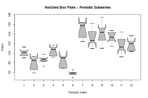
Figures (Output of Computation) | |||||||||||||||||||||
Input Parameters & R Code | |||||||||||||||||||||
| Parameters (Session): | |||||||||||||||||||||
| par1 = 12 ; | |||||||||||||||||||||
| Parameters (R input): | |||||||||||||||||||||
| par1 = 12 ; | |||||||||||||||||||||
| R code (references can be found in the software module): | |||||||||||||||||||||
par1 <- as.numeric(par1) | |||||||||||||||||||||