Repository of Reproducible Computations

Free Statistics

of Irreproducible Research!

Author's title

Author

*Unverified author*

R Software Module

rwasp_autocorrelation.wasp

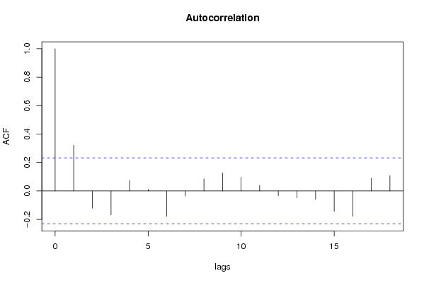
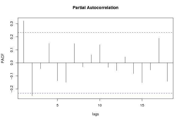
Title produced by software

(Partial) Autocorrelation Function

Date of computation

Tue, 11 Dec 2007 12:01:13 -0700

Cite this page as follows

Statistical Computations at FreeStatistics.org, Office for Research Development and Education, URL https://freestatistics.org/blog/index.php?v=date/2007/Dec/11/t1197398834yg3hnw71sh0h3xg.htm/, Retrieved Mon, 29 Apr 2024 05:14:19 +0000

Statistical Computations at FreeStatistics.org, Office for Research Development and Education, URL https://freestatistics.org/blog/index.php?pk=3146, Retrieved Mon, 29 Apr 2024 05:14:19 +0000

QR Codes:

Paste this QR Code to cite your computation.

Original text written by user:

IsPrivate?

No (this computation is public)

User-defined keywords

Estimated Impact

215

Family? (F = Feedback message, R = changed R code, M = changed R Module, P = changed Parameters, D = changed Data)

-       [(Partial) Autocorrelation Function] [Inducing stationa...] [2007-12-11 19:01:13] [578856645eee7b4b8f74dcf589866e9b] [Current]

Feedback Forum

Post a new message

Dataseries X:

Download CSV

Histogram

Boxplots

Summary of compuational transaction
Raw Input	view raw input (R code)
Raw Output	view raw output of R engine
Computing time	1 seconds
R Server	'Gwilym Jenkins' @ 72.249.127.135

\begin{tabular}{lllllllll}
\hline
Summary of compuational transaction \tabularnewline
Raw Input & view raw input (R code)  \tabularnewline
Raw Output & view raw output of R engine  \tabularnewline
Computing time & 1 seconds \tabularnewline
R Server & 'Gwilym Jenkins' @ 72.249.127.135 \tabularnewline
\hline
\end{tabular}
%Source: https://freestatistics.org/blog/index.php?pk=3146&T=0

[TABLE]
[ROW][C]Summary of compuational transaction[/C][/ROW]
[ROW][C]Raw Input[/C][C]view raw input (R code) [/C][/ROW]
[ROW][C]Raw Output[/C][C]view raw output of R engine [/C][/ROW]
[ROW][C]Computing time[/C][C]1 seconds[/C][/ROW]
[ROW][C]R Server[/C][C]'Gwilym Jenkins' @ 72.249.127.135[/C][/ROW]
[/TABLE]
Source: https://freestatistics.org/blog/index.php?pk=3146&T=0

Globally Unique Identifier (entire table): ba.freestatistics.org/blog/index.php?pk=3146&T=0

As an alternative you can also use a QR Code:

The GUIDs for individual cells are displayed in the table below:

Summary of compuational transaction
Raw Input	view raw input (R code)
Raw Output	view raw output of R engine
Computing time	1 seconds
R Server	'Gwilym Jenkins' @ 72.249.127.135

Autocorrelation Function
Time lag k	ACF(k)	T-STAT	P-value
0	1	8.4261	0
1	0.322329	2.716	0.004146
2	-0.122287	-1.0304	0.846842
3	-0.16786	-1.4144	0.919194
4	0.073396	0.6184	0.26913
5	0.010908	0.0919	0.463512
6	-0.178697	-1.5057	0.931713
7	-0.035679	-0.3006	0.617715
8	0.085422	0.7198	0.237012
9	0.126405	1.0651	0.145219
10	0.096629	0.8142	0.209124
11	0.039735	0.3348	0.369378
12	-0.033394	-0.2814	0.610381
13	-0.049338	-0.4157	0.660568
14	-0.057889	-0.4878	0.686396
15	-0.143305	-1.2075	0.884378
16	-0.178032	-1.5001	0.930992
17	0.089338	0.7528	0.227037

\begin{tabular}{lllllllll}
\hline
Autocorrelation Function \tabularnewline
Time lag k & ACF(k) & T-STAT & P-value \tabularnewline
0 & 1 & 8.4261 & 0 \tabularnewline
1 & 0.322329 & 2.716 & 0.004146 \tabularnewline
2 & -0.122287 & -1.0304 & 0.846842 \tabularnewline
3 & -0.16786 & -1.4144 & 0.919194 \tabularnewline
4 & 0.073396 & 0.6184 & 0.26913 \tabularnewline
5 & 0.010908 & 0.0919 & 0.463512 \tabularnewline
6 & -0.178697 & -1.5057 & 0.931713 \tabularnewline
7 & -0.035679 & -0.3006 & 0.617715 \tabularnewline
8 & 0.085422 & 0.7198 & 0.237012 \tabularnewline
9 & 0.126405 & 1.0651 & 0.145219 \tabularnewline
10 & 0.096629 & 0.8142 & 0.209124 \tabularnewline
11 & 0.039735 & 0.3348 & 0.369378 \tabularnewline
12 & -0.033394 & -0.2814 & 0.610381 \tabularnewline
13 & -0.049338 & -0.4157 & 0.660568 \tabularnewline
14 & -0.057889 & -0.4878 & 0.686396 \tabularnewline
15 & -0.143305 & -1.2075 & 0.884378 \tabularnewline
16 & -0.178032 & -1.5001 & 0.930992 \tabularnewline
17 & 0.089338 & 0.7528 & 0.227037 \tabularnewline
\hline
\end{tabular}
%Source: https://freestatistics.org/blog/index.php?pk=3146&T=1

[TABLE]
[ROW][C]Autocorrelation Function[/C][/ROW]
[ROW][C]Time lag k[/C][C]ACF(k)[/C][C]T-STAT[/C][C]P-value[/C][/ROW]
[ROW][C]0[/C][C]1[/C][C]8.4261[/C][C]0[/C][/ROW]
[ROW][C]1[/C][C]0.322329[/C][C]2.716[/C][C]0.004146[/C][/ROW]
[ROW][C]2[/C][C]-0.122287[/C][C]-1.0304[/C][C]0.846842[/C][/ROW]
[ROW][C]3[/C][C]-0.16786[/C][C]-1.4144[/C][C]0.919194[/C][/ROW]
[ROW][C]4[/C][C]0.073396[/C][C]0.6184[/C][C]0.26913[/C][/ROW]
[ROW][C]5[/C][C]0.010908[/C][C]0.0919[/C][C]0.463512[/C][/ROW]
[ROW][C]6[/C][C]-0.178697[/C][C]-1.5057[/C][C]0.931713[/C][/ROW]
[ROW][C]7[/C][C]-0.035679[/C][C]-0.3006[/C][C]0.617715[/C][/ROW]
[ROW][C]8[/C][C]0.085422[/C][C]0.7198[/C][C]0.237012[/C][/ROW]
[ROW][C]9[/C][C]0.126405[/C][C]1.0651[/C][C]0.145219[/C][/ROW]
[ROW][C]10[/C][C]0.096629[/C][C]0.8142[/C][C]0.209124[/C][/ROW]
[ROW][C]11[/C][C]0.039735[/C][C]0.3348[/C][C]0.369378[/C][/ROW]
[ROW][C]12[/C][C]-0.033394[/C][C]-0.2814[/C][C]0.610381[/C][/ROW]
[ROW][C]13[/C][C]-0.049338[/C][C]-0.4157[/C][C]0.660568[/C][/ROW]
[ROW][C]14[/C][C]-0.057889[/C][C]-0.4878[/C][C]0.686396[/C][/ROW]
[ROW][C]15[/C][C]-0.143305[/C][C]-1.2075[/C][C]0.884378[/C][/ROW]
[ROW][C]16[/C][C]-0.178032[/C][C]-1.5001[/C][C]0.930992[/C][/ROW]
[ROW][C]17[/C][C]0.089338[/C][C]0.7528[/C][C]0.227037[/C][/ROW]
[/TABLE]
Source: https://freestatistics.org/blog/index.php?pk=3146&T=1

Globally Unique Identifier (entire table): ba.freestatistics.org/blog/index.php?pk=3146&T=1

As an alternative you can also use a QR Code:

The GUIDs for individual cells are displayed in the table below:

Autocorrelation Function
Time lag k	ACF(k)	T-STAT	P-value
0	1	8.4261	0
1	0.322329	2.716	0.004146
2	-0.122287	-1.0304	0.846842
3	-0.16786	-1.4144	0.919194
4	0.073396	0.6184	0.26913
5	0.010908	0.0919	0.463512
6	-0.178697	-1.5057	0.931713
7	-0.035679	-0.3006	0.617715
8	0.085422	0.7198	0.237012
9	0.126405	1.0651	0.145219
10	0.096629	0.8142	0.209124
11	0.039735	0.3348	0.369378
12	-0.033394	-0.2814	0.610381
13	-0.049338	-0.4157	0.660568
14	-0.057889	-0.4878	0.686396
15	-0.143305	-1.2075	0.884378
16	-0.178032	-1.5001	0.930992
17	0.089338	0.7528	0.227037

Partial Autocorrelation Function
Time lag k	PACF(k)	T-STAT	P-value
0	0.322329	2.716	0.004146
1	-0.252407	-2.1268	0.981544
2	-0.044262	-0.373	0.644853
3	0.149121	1.2565	0.106524
4	-0.137429	-1.158	0.874627
5	-0.149645	-1.2609	0.89427
6	0.14847	1.251	0.107515
7	-0.03126	-0.2634	0.603496
8	0.062098	0.5233	0.301215
9	0.139695	1.1771	0.121544
10	-0.034059	-0.287	0.612522
11	-0.058333	-0.4915	0.687714
12	0.046044	0.388	0.349599
13	-0.082212	-0.6927	0.754631
14	-0.151355	-1.2753	0.896827
15	-0.055078	-0.4641	0.678002
16	0.189326	1.5953	0.057545
17	-0.142603	-1.2016	0.883243

\begin{tabular}{lllllllll}
\hline
Partial Autocorrelation Function \tabularnewline
Time lag k & PACF(k) & T-STAT & P-value \tabularnewline
0 & 0.322329 & 2.716 & 0.004146 \tabularnewline
1 & -0.252407 & -2.1268 & 0.981544 \tabularnewline
2 & -0.044262 & -0.373 & 0.644853 \tabularnewline
3 & 0.149121 & 1.2565 & 0.106524 \tabularnewline
4 & -0.137429 & -1.158 & 0.874627 \tabularnewline
5 & -0.149645 & -1.2609 & 0.89427 \tabularnewline
6 & 0.14847 & 1.251 & 0.107515 \tabularnewline
7 & -0.03126 & -0.2634 & 0.603496 \tabularnewline
8 & 0.062098 & 0.5233 & 0.301215 \tabularnewline
9 & 0.139695 & 1.1771 & 0.121544 \tabularnewline
10 & -0.034059 & -0.287 & 0.612522 \tabularnewline
11 & -0.058333 & -0.4915 & 0.687714 \tabularnewline
12 & 0.046044 & 0.388 & 0.349599 \tabularnewline
13 & -0.082212 & -0.6927 & 0.754631 \tabularnewline
14 & -0.151355 & -1.2753 & 0.896827 \tabularnewline
15 & -0.055078 & -0.4641 & 0.678002 \tabularnewline
16 & 0.189326 & 1.5953 & 0.057545 \tabularnewline
17 & -0.142603 & -1.2016 & 0.883243 \tabularnewline
\hline
\end{tabular}
%Source: https://freestatistics.org/blog/index.php?pk=3146&T=2

[TABLE]
[ROW][C]Partial Autocorrelation Function[/C][/ROW]
[ROW][C]Time lag k[/C][C]PACF(k)[/C][C]T-STAT[/C][C]P-value[/C][/ROW]
[ROW][C]0[/C][C]0.322329[/C][C]2.716[/C][C]0.004146[/C][/ROW]
[ROW][C]1[/C][C]-0.252407[/C][C]-2.1268[/C][C]0.981544[/C][/ROW]
[ROW][C]2[/C][C]-0.044262[/C][C]-0.373[/C][C]0.644853[/C][/ROW]
[ROW][C]3[/C][C]0.149121[/C][C]1.2565[/C][C]0.106524[/C][/ROW]
[ROW][C]4[/C][C]-0.137429[/C][C]-1.158[/C][C]0.874627[/C][/ROW]
[ROW][C]5[/C][C]-0.149645[/C][C]-1.2609[/C][C]0.89427[/C][/ROW]
[ROW][C]6[/C][C]0.14847[/C][C]1.251[/C][C]0.107515[/C][/ROW]
[ROW][C]7[/C][C]-0.03126[/C][C]-0.2634[/C][C]0.603496[/C][/ROW]
[ROW][C]8[/C][C]0.062098[/C][C]0.5233[/C][C]0.301215[/C][/ROW]
[ROW][C]9[/C][C]0.139695[/C][C]1.1771[/C][C]0.121544[/C][/ROW]
[ROW][C]10[/C][C]-0.034059[/C][C]-0.287[/C][C]0.612522[/C][/ROW]
[ROW][C]11[/C][C]-0.058333[/C][C]-0.4915[/C][C]0.687714[/C][/ROW]
[ROW][C]12[/C][C]0.046044[/C][C]0.388[/C][C]0.349599[/C][/ROW]
[ROW][C]13[/C][C]-0.082212[/C][C]-0.6927[/C][C]0.754631[/C][/ROW]
[ROW][C]14[/C][C]-0.151355[/C][C]-1.2753[/C][C]0.896827[/C][/ROW]
[ROW][C]15[/C][C]-0.055078[/C][C]-0.4641[/C][C]0.678002[/C][/ROW]
[ROW][C]16[/C][C]0.189326[/C][C]1.5953[/C][C]0.057545[/C][/ROW]
[ROW][C]17[/C][C]-0.142603[/C][C]-1.2016[/C][C]0.883243[/C][/ROW]
[/TABLE]
Source: https://freestatistics.org/blog/index.php?pk=3146&T=2

Globally Unique Identifier (entire table): ba.freestatistics.org/blog/index.php?pk=3146&T=2

As an alternative you can also use a QR Code:

The GUIDs for individual cells are displayed in the table below:

Partial Autocorrelation Function
Time lag k	PACF(k)	T-STAT	P-value
0	0.322329	2.716	0.004146
1	-0.252407	-2.1268	0.981544
2	-0.044262	-0.373	0.644853
3	0.149121	1.2565	0.106524
4	-0.137429	-1.158	0.874627
5	-0.149645	-1.2609	0.89427
6	0.14847	1.251	0.107515
7	-0.03126	-0.2634	0.603496
8	0.062098	0.5233	0.301215
9	0.139695	1.1771	0.121544
10	-0.034059	-0.287	0.612522
11	-0.058333	-0.4915	0.687714
12	0.046044	0.388	0.349599
13	-0.082212	-0.6927	0.754631
14	-0.151355	-1.2753	0.896827
15	-0.055078	-0.4641	0.678002
16	0.189326	1.5953	0.057545
17	-0.142603	-1.2016	0.883243

Figure 1

PNG link

Postscript link

PDF link

Figure 2

PNG link

Postscript link

PDF link

Parameters (Session):

par1 = Default ; par2 = 1 ; par3 = 1 ; par4 = 0 ; par5 = 12 ;

Parameters (R input):

par1 = Default ; par2 = 1 ; par3 = 1 ; par4 = 0 ; par5 = 12 ;

R code (references can be found in the software module):

if (par1 == 'Default') {
par1 = 10*log10(length(x))
} else {
par1 <- as.numeric(par1)
}
par2 <- as.numeric(par2)
par3 <- as.numeric(par3)
par4 <- as.numeric(par4)
par5 <- as.numeric(par5)
if (par2 == 0) {
x <- log(x)
} else {
x <- (x ^ par2 - 1) / par2
}
if (par3 > 0) x <- diff(x,lag=1,difference=par3)
if (par4 > 0) x <- diff(x,lag=par5,difference=par4)
bitmap(file='pic1.png')
racf <- acf(x,par1,main='Autocorrelation',xlab='lags',ylab='ACF')
dev.off()
bitmap(file='pic2.png')
rpacf <- pacf(x,par1,main='Partial Autocorrelation',xlab='lags',ylab='PACF')
dev.off()
(myacf <- c(racf$acf))
(mypacf <- c(rpacf$acf))
lengthx <- length(x)
sqrtn <- sqrt(lengthx)
load(file='createtable')
a<-table.start()
a<-table.row.start(a)
a<-table.element(a,'Autocorrelation Function',4,TRUE)
a<-table.row.end(a)
a<-table.row.start(a)
a<-table.element(a,'Time lag k',header=TRUE)
a<-table.element(a,hyperlink('basics.htm','ACF(k)','click here for more information about the Autocorrelation Function'),header=TRUE)
a<-table.element(a,'T-STAT',header=TRUE)
a<-table.element(a,'P-value',header=TRUE)
a<-table.row.end(a)
for (i in 1:par1) {
a<-table.row.start(a)
a<-table.element(a,i-1,header=TRUE)
a<-table.element(a,round(myacf[i],6))
mytstat <- myacf[i]*sqrtn
a<-table.element(a,round(mytstat,4))
a<-table.element(a,round(1-pt(mytstat,lengthx),6))
a<-table.row.end(a)
}
a<-table.end(a)
table.save(a,file='mytable.tab')
a<-table.start()
a<-table.row.start(a)
a<-table.element(a,'Partial Autocorrelation Function',4,TRUE)
a<-table.row.end(a)
a<-table.row.start(a)
a<-table.element(a,'Time lag k',header=TRUE)
a<-table.element(a,hyperlink('basics.htm','PACF(k)','click here for more information about the Partial Autocorrelation Function'),header=TRUE)
a<-table.element(a,'T-STAT',header=TRUE)
a<-table.element(a,'P-value',header=TRUE)
a<-table.row.end(a)
for (i in 1:par1) {
a<-table.row.start(a)
a<-table.element(a,i-1,header=TRUE)
a<-table.element(a,round(mypacf[i],6))
mytstat <- mypacf[i]*sqrtn
a<-table.element(a,round(mytstat,4))
a<-table.element(a,round(1-pt(mytstat,lengthx),6))
a<-table.row.end(a)
}
a<-table.end(a)
table.save(a,file='mytable1.tab')

Free Statistics

Description of Statistical Computation

Tree of Dependent Computations

Dataset

Tables (Output of Computation)

Figures (Output of Computation)

Input Parameters & R Code