Repository of Reproducible Computations

Free Statistics

of Irreproducible Research!

Author's title

Author

*Unverified author*

R Software Module

rwasp_autocorrelation.wasp

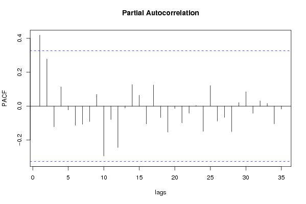
Title produced by software

(Partial) Autocorrelation Function

Date of computation

Mon, 10 Dec 2007 12:52:13 -0700

Cite this page as follows

Statistical Computations at FreeStatistics.org, Office for Research Development and Education, URL https://freestatistics.org/blog/index.php?v=date/2007/Dec/10/t1197315514f5l5ets6a1r9iiq.htm/, Retrieved Tue, 07 May 2024 03:06:08 +0000

Statistical Computations at FreeStatistics.org, Office for Research Development and Education, URL https://freestatistics.org/blog/index.php?pk=3028, Retrieved Tue, 07 May 2024 03:06:08 +0000

QR Codes:

Paste this QR Code to cite your computation.

Original text written by user:

IsPrivate?

No (this computation is public)

User-defined keywords

Lise Swinnen

Estimated Impact

197

Family? (F = Feedback message, R = changed R code, M = changed R Module, P = changed Parameters, D = changed Data)

-       [(Partial) Autocorrelation Function] [paper (acf/vrm 2)] [2007-12-10 19:52:13] [a526d213baffe7453818dd375c9a7100] [Current]

Feedback Forum

Post a new message

Dataseries X:

Download CSV

Histogram

Boxplots

0,007850049
0,008671912
0,008391986
0,008691954
0,008724839
0,008949762
0,009344295
0,009971514
0,010388067
0,008884599
0,01000981
0,012393539
0,007933519
0,008087396
0,008120881
0,008147148
0,00917087
0,009668358
0,009897495
0,011217878
0,010190084
0,009560637
0,011200671
0,013546776
0,008524882
0,009142143
0,008793047
0,009296235
0,009974995
0,009692013
0,010120046
0,011004981
0,010328492
0,009428406
0,011114429
0,011798579
0,008997058
0,008803914
0,007974159
0,008460945
0,009917747
0,009604284
0,011028851
0,011162991
0,010420855
0,009897095
0,010715298
0,012461041
0,008754735
0,009381664
0,008843755
0,009235122
0,009973356
0,009146341
0,011038445
0,010830104
0,010585414
0,010560523
0,010897526
0,014012667

Summary of compuational transaction
Raw Input	view raw input (R code)
Raw Output	view raw output of R engine
Computing time	1 seconds
R Server	'Gwilym Jenkins' @ 72.249.127.135

\begin{tabular}{lllllllll}
\hline
Summary of compuational transaction \tabularnewline
Raw Input & view raw input (R code)  \tabularnewline
Raw Output & view raw output of R engine  \tabularnewline
Computing time & 1 seconds \tabularnewline
R Server & 'Gwilym Jenkins' @ 72.249.127.135 \tabularnewline
\hline
\end{tabular}
%Source: https://freestatistics.org/blog/index.php?pk=3028&T=0

[TABLE]
[ROW][C]Summary of compuational transaction[/C][/ROW]
[ROW][C]Raw Input[/C][C]view raw input (R code) [/C][/ROW]
[ROW][C]Raw Output[/C][C]view raw output of R engine [/C][/ROW]
[ROW][C]Computing time[/C][C]1 seconds[/C][/ROW]
[ROW][C]R Server[/C][C]'Gwilym Jenkins' @ 72.249.127.135[/C][/ROW]
[/TABLE]
Source: https://freestatistics.org/blog/index.php?pk=3028&T=0

Globally Unique Identifier (entire table): ba.freestatistics.org/blog/index.php?pk=3028&T=0

As an alternative you can also use a QR Code:

The GUIDs for individual cells are displayed in the table below:

Summary of compuational transaction
Raw Input	view raw input (R code)
Raw Output	view raw output of R engine
Computing time	1 seconds
R Server	'Gwilym Jenkins' @ 72.249.127.135

Autocorrelation Function
Time lag k	ACF(k)	T-STAT	P-value
0	1	6	0
1	0.418329	2.51	0.008355
2	0.404448	2.4267	0.010186
3	0.145815	0.8749	0.193716
4	0.210897	1.2654	0.106931
5	0.080598	0.4836	0.315804
6	0.019842	0.1191	0.452947
7	-0.101998	-0.612	0.727803
8	-0.146804	-0.8808	0.807872
9	-0.087665	-0.526	0.698939
10	-0.301047	-1.8063	0.96038
11	-0.256605	-1.5396	0.933803
12	-0.462414	-2.7745	0.995645
13	-0.278457	-1.6707	0.948277
14	-0.224391	-1.3463	0.906696
15	-0.065163	-0.391	0.650942
16	-0.166585	-0.9995	0.837891
17	0.018706	0.1122	0.45563
18	-0.0236	-0.1416	0.555908
19	0.000133	8e-04	0.499684
20	0.020791	0.1247	0.45071
21	-0.039695	-0.2382	0.593449
22	0.062577	0.3755	0.35476
23	0.077748	0.4665	0.321838
24	0.073922	0.4435	0.330018
25	0.089464	0.5368	0.29736
26	0.050094	0.3006	0.382739
27	-0.035813	-0.2149	0.584464
28	-0.083408	-0.5004	0.690098
29	-0.056425	-0.3386	0.631543
30	-0.026156	-0.1569	0.561914
31	0.032551	0.1953	0.423127
32	0.055891	0.3353	0.369656
33	0.043693	0.2622	0.397347
34	0.040185	0.2411	0.405418
35	0.010543	0.0633	0.474955
36	NA	NA	NA
37	NA	NA	NA
38	NA	NA	NA
39	NA	NA	NA
40	NA	NA	NA
41	NA	NA	NA
42	NA	NA	NA
43	NA	NA	NA
44	NA	NA	NA
45	NA	NA	NA
46	NA	NA	NA
47	NA	NA	NA

\begin{tabular}{lllllllll}
\hline
Autocorrelation Function \tabularnewline
Time lag k & ACF(k) & T-STAT & P-value \tabularnewline
0 & 1 & 6 & 0 \tabularnewline
1 & 0.418329 & 2.51 & 0.008355 \tabularnewline
2 & 0.404448 & 2.4267 & 0.010186 \tabularnewline
3 & 0.145815 & 0.8749 & 0.193716 \tabularnewline
4 & 0.210897 & 1.2654 & 0.106931 \tabularnewline
5 & 0.080598 & 0.4836 & 0.315804 \tabularnewline
6 & 0.019842 & 0.1191 & 0.452947 \tabularnewline
7 & -0.101998 & -0.612 & 0.727803 \tabularnewline
8 & -0.146804 & -0.8808 & 0.807872 \tabularnewline
9 & -0.087665 & -0.526 & 0.698939 \tabularnewline
10 & -0.301047 & -1.8063 & 0.96038 \tabularnewline
11 & -0.256605 & -1.5396 & 0.933803 \tabularnewline
12 & -0.462414 & -2.7745 & 0.995645 \tabularnewline
13 & -0.278457 & -1.6707 & 0.948277 \tabularnewline
14 & -0.224391 & -1.3463 & 0.906696 \tabularnewline
15 & -0.065163 & -0.391 & 0.650942 \tabularnewline
16 & -0.166585 & -0.9995 & 0.837891 \tabularnewline
17 & 0.018706 & 0.1122 & 0.45563 \tabularnewline
18 & -0.0236 & -0.1416 & 0.555908 \tabularnewline
19 & 0.000133 & 8e-04 & 0.499684 \tabularnewline
20 & 0.020791 & 0.1247 & 0.45071 \tabularnewline
21 & -0.039695 & -0.2382 & 0.593449 \tabularnewline
22 & 0.062577 & 0.3755 & 0.35476 \tabularnewline
23 & 0.077748 & 0.4665 & 0.321838 \tabularnewline
24 & 0.073922 & 0.4435 & 0.330018 \tabularnewline
25 & 0.089464 & 0.5368 & 0.29736 \tabularnewline
26 & 0.050094 & 0.3006 & 0.382739 \tabularnewline
27 & -0.035813 & -0.2149 & 0.584464 \tabularnewline
28 & -0.083408 & -0.5004 & 0.690098 \tabularnewline
29 & -0.056425 & -0.3386 & 0.631543 \tabularnewline
30 & -0.026156 & -0.1569 & 0.561914 \tabularnewline
31 & 0.032551 & 0.1953 & 0.423127 \tabularnewline
32 & 0.055891 & 0.3353 & 0.369656 \tabularnewline
33 & 0.043693 & 0.2622 & 0.397347 \tabularnewline
34 & 0.040185 & 0.2411 & 0.405418 \tabularnewline
35 & 0.010543 & 0.0633 & 0.474955 \tabularnewline
36 & NA & NA & NA \tabularnewline
37 & NA & NA & NA \tabularnewline
38 & NA & NA & NA \tabularnewline
39 & NA & NA & NA \tabularnewline
40 & NA & NA & NA \tabularnewline
41 & NA & NA & NA \tabularnewline
42 & NA & NA & NA \tabularnewline
43 & NA & NA & NA \tabularnewline
44 & NA & NA & NA \tabularnewline
45 & NA & NA & NA \tabularnewline
46 & NA & NA & NA \tabularnewline
47 & NA & NA & NA \tabularnewline
\hline
\end{tabular}
%Source: https://freestatistics.org/blog/index.php?pk=3028&T=1

[TABLE]
[ROW][C]Autocorrelation Function[/C][/ROW]
[ROW][C]Time lag k[/C][C]ACF(k)[/C][C]T-STAT[/C][C]P-value[/C][/ROW]
[ROW][C]0[/C][C]1[/C][C]6[/C][C]0[/C][/ROW]
[ROW][C]1[/C][C]0.418329[/C][C]2.51[/C][C]0.008355[/C][/ROW]
[ROW][C]2[/C][C]0.404448[/C][C]2.4267[/C][C]0.010186[/C][/ROW]
[ROW][C]3[/C][C]0.145815[/C][C]0.8749[/C][C]0.193716[/C][/ROW]
[ROW][C]4[/C][C]0.210897[/C][C]1.2654[/C][C]0.106931[/C][/ROW]
[ROW][C]5[/C][C]0.080598[/C][C]0.4836[/C][C]0.315804[/C][/ROW]
[ROW][C]6[/C][C]0.019842[/C][C]0.1191[/C][C]0.452947[/C][/ROW]
[ROW][C]7[/C][C]-0.101998[/C][C]-0.612[/C][C]0.727803[/C][/ROW]
[ROW][C]8[/C][C]-0.146804[/C][C]-0.8808[/C][C]0.807872[/C][/ROW]
[ROW][C]9[/C][C]-0.087665[/C][C]-0.526[/C][C]0.698939[/C][/ROW]
[ROW][C]10[/C][C]-0.301047[/C][C]-1.8063[/C][C]0.96038[/C][/ROW]
[ROW][C]11[/C][C]-0.256605[/C][C]-1.5396[/C][C]0.933803[/C][/ROW]
[ROW][C]12[/C][C]-0.462414[/C][C]-2.7745[/C][C]0.995645[/C][/ROW]
[ROW][C]13[/C][C]-0.278457[/C][C]-1.6707[/C][C]0.948277[/C][/ROW]
[ROW][C]14[/C][C]-0.224391[/C][C]-1.3463[/C][C]0.906696[/C][/ROW]
[ROW][C]15[/C][C]-0.065163[/C][C]-0.391[/C][C]0.650942[/C][/ROW]
[ROW][C]16[/C][C]-0.166585[/C][C]-0.9995[/C][C]0.837891[/C][/ROW]
[ROW][C]17[/C][C]0.018706[/C][C]0.1122[/C][C]0.45563[/C][/ROW]
[ROW][C]18[/C][C]-0.0236[/C][C]-0.1416[/C][C]0.555908[/C][/ROW]
[ROW][C]19[/C][C]0.000133[/C][C]8e-04[/C][C]0.499684[/C][/ROW]
[ROW][C]20[/C][C]0.020791[/C][C]0.1247[/C][C]0.45071[/C][/ROW]
[ROW][C]21[/C][C]-0.039695[/C][C]-0.2382[/C][C]0.593449[/C][/ROW]
[ROW][C]22[/C][C]0.062577[/C][C]0.3755[/C][C]0.35476[/C][/ROW]
[ROW][C]23[/C][C]0.077748[/C][C]0.4665[/C][C]0.321838[/C][/ROW]
[ROW][C]24[/C][C]0.073922[/C][C]0.4435[/C][C]0.330018[/C][/ROW]
[ROW][C]25[/C][C]0.089464[/C][C]0.5368[/C][C]0.29736[/C][/ROW]
[ROW][C]26[/C][C]0.050094[/C][C]0.3006[/C][C]0.382739[/C][/ROW]
[ROW][C]27[/C][C]-0.035813[/C][C]-0.2149[/C][C]0.584464[/C][/ROW]
[ROW][C]28[/C][C]-0.083408[/C][C]-0.5004[/C][C]0.690098[/C][/ROW]
[ROW][C]29[/C][C]-0.056425[/C][C]-0.3386[/C][C]0.631543[/C][/ROW]
[ROW][C]30[/C][C]-0.026156[/C][C]-0.1569[/C][C]0.561914[/C][/ROW]
[ROW][C]31[/C][C]0.032551[/C][C]0.1953[/C][C]0.423127[/C][/ROW]
[ROW][C]32[/C][C]0.055891[/C][C]0.3353[/C][C]0.369656[/C][/ROW]
[ROW][C]33[/C][C]0.043693[/C][C]0.2622[/C][C]0.397347[/C][/ROW]
[ROW][C]34[/C][C]0.040185[/C][C]0.2411[/C][C]0.405418[/C][/ROW]
[ROW][C]35[/C][C]0.010543[/C][C]0.0633[/C][C]0.474955[/C][/ROW]
[ROW][C]36[/C][C]NA[/C][C]NA[/C][C]NA[/C][/ROW]
[ROW][C]37[/C][C]NA[/C][C]NA[/C][C]NA[/C][/ROW]
[ROW][C]38[/C][C]NA[/C][C]NA[/C][C]NA[/C][/ROW]
[ROW][C]39[/C][C]NA[/C][C]NA[/C][C]NA[/C][/ROW]
[ROW][C]40[/C][C]NA[/C][C]NA[/C][C]NA[/C][/ROW]
[ROW][C]41[/C][C]NA[/C][C]NA[/C][C]NA[/C][/ROW]
[ROW][C]42[/C][C]NA[/C][C]NA[/C][C]NA[/C][/ROW]
[ROW][C]43[/C][C]NA[/C][C]NA[/C][C]NA[/C][/ROW]
[ROW][C]44[/C][C]NA[/C][C]NA[/C][C]NA[/C][/ROW]
[ROW][C]45[/C][C]NA[/C][C]NA[/C][C]NA[/C][/ROW]
[ROW][C]46[/C][C]NA[/C][C]NA[/C][C]NA[/C][/ROW]
[ROW][C]47[/C][C]NA[/C][C]NA[/C][C]NA[/C][/ROW]
[/TABLE]
Source: https://freestatistics.org/blog/index.php?pk=3028&T=1

Globally Unique Identifier (entire table): ba.freestatistics.org/blog/index.php?pk=3028&T=1

As an alternative you can also use a QR Code:

The GUIDs for individual cells are displayed in the table below:

Autocorrelation Function
Time lag k	ACF(k)	T-STAT	P-value
0	1	6	0
1	0.418329	2.51	0.008355
2	0.404448	2.4267	0.010186
3	0.145815	0.8749	0.193716
4	0.210897	1.2654	0.106931
5	0.080598	0.4836	0.315804
6	0.019842	0.1191	0.452947
7	-0.101998	-0.612	0.727803
8	-0.146804	-0.8808	0.807872
9	-0.087665	-0.526	0.698939
10	-0.301047	-1.8063	0.96038
11	-0.256605	-1.5396	0.933803
12	-0.462414	-2.7745	0.995645
13	-0.278457	-1.6707	0.948277
14	-0.224391	-1.3463	0.906696
15	-0.065163	-0.391	0.650942
16	-0.166585	-0.9995	0.837891
17	0.018706	0.1122	0.45563
18	-0.0236	-0.1416	0.555908
19	0.000133	8e-04	0.499684
20	0.020791	0.1247	0.45071
21	-0.039695	-0.2382	0.593449
22	0.062577	0.3755	0.35476
23	0.077748	0.4665	0.321838
24	0.073922	0.4435	0.330018
25	0.089464	0.5368	0.29736
26	0.050094	0.3006	0.382739
27	-0.035813	-0.2149	0.584464
28	-0.083408	-0.5004	0.690098
29	-0.056425	-0.3386	0.631543
30	-0.026156	-0.1569	0.561914
31	0.032551	0.1953	0.423127
32	0.055891	0.3353	0.369656
33	0.043693	0.2622	0.397347
34	0.040185	0.2411	0.405418
35	0.010543	0.0633	0.474955
36	NA	NA	NA
37	NA	NA	NA
38	NA	NA	NA
39	NA	NA	NA
40	NA	NA	NA
41	NA	NA	NA
42	NA	NA	NA
43	NA	NA	NA
44	NA	NA	NA
45	NA	NA	NA
46	NA	NA	NA
47	NA	NA	NA

Partial Autocorrelation Function
Time lag k	PACF(k)	T-STAT	P-value
0	0.418329	2.51	0.008355
1	0.27812	1.6687	0.051924
2	-0.121741	-0.7304	0.765077
3	0.114014	0.6841	0.24915
4	-0.02271	-0.1363	0.553812
5	-0.113598	-0.6816	0.75007
6	-0.106781	-0.6407	0.737107
7	-0.090938	-0.5456	0.705656
8	0.069064	0.4144	0.340526
9	-0.294388	-1.7663	0.95709
10	-0.079234	-0.4754	0.681315
11	-0.244593	-1.4676	0.924547
12	-0.01183	-0.071	0.528097
13	0.127058	0.7623	0.225409
14	0.063737	0.3824	0.352197
15	-0.104494	-0.627	0.73268
16	0.124686	0.7481	0.229625
17	-0.067519	-0.4051	0.656105
18	-0.153544	-0.9213	0.818477
19	-0.013957	-0.0837	0.533137
20	-0.099109	-0.5947	0.722103
21	-0.041752	-0.2505	0.598193
22	0.003754	0.0225	0.491077
23	-0.148433	-0.8906	0.810471
24	0.120888	0.7253	0.236469
25	-0.088275	-0.5297	0.700198
26	-0.066445	-0.3987	0.653754
27	-0.150568	-0.9034	0.813843
28	0.021128	0.1268	0.449916
29	0.084443	0.5067	0.307742
30	-0.042458	-0.2548	0.599817
31	0.030876	0.1853	0.427034
32	0.015891	0.0953	0.462284
33	-0.105149	-0.6309	0.733953
34	-0.017764	-0.1066	0.542146
35	NA	NA	NA
36	NA	NA	NA
37	NA	NA	NA
38	NA	NA	NA
39	NA	NA	NA
40	NA	NA	NA
41	NA	NA	NA
42	NA	NA	NA
43	NA	NA	NA
44	NA	NA	NA
45	NA	NA	NA
46	NA	NA	NA
47	NA	NA	NA

\begin{tabular}{lllllllll}
\hline
Partial Autocorrelation Function \tabularnewline
Time lag k & PACF(k) & T-STAT & P-value \tabularnewline
0 & 0.418329 & 2.51 & 0.008355 \tabularnewline
1 & 0.27812 & 1.6687 & 0.051924 \tabularnewline
2 & -0.121741 & -0.7304 & 0.765077 \tabularnewline
3 & 0.114014 & 0.6841 & 0.24915 \tabularnewline
4 & -0.02271 & -0.1363 & 0.553812 \tabularnewline
5 & -0.113598 & -0.6816 & 0.75007 \tabularnewline
6 & -0.106781 & -0.6407 & 0.737107 \tabularnewline
7 & -0.090938 & -0.5456 & 0.705656 \tabularnewline
8 & 0.069064 & 0.4144 & 0.340526 \tabularnewline
9 & -0.294388 & -1.7663 & 0.95709 \tabularnewline
10 & -0.079234 & -0.4754 & 0.681315 \tabularnewline
11 & -0.244593 & -1.4676 & 0.924547 \tabularnewline
12 & -0.01183 & -0.071 & 0.528097 \tabularnewline
13 & 0.127058 & 0.7623 & 0.225409 \tabularnewline
14 & 0.063737 & 0.3824 & 0.352197 \tabularnewline
15 & -0.104494 & -0.627 & 0.73268 \tabularnewline
16 & 0.124686 & 0.7481 & 0.229625 \tabularnewline
17 & -0.067519 & -0.4051 & 0.656105 \tabularnewline
18 & -0.153544 & -0.9213 & 0.818477 \tabularnewline
19 & -0.013957 & -0.0837 & 0.533137 \tabularnewline
20 & -0.099109 & -0.5947 & 0.722103 \tabularnewline
21 & -0.041752 & -0.2505 & 0.598193 \tabularnewline
22 & 0.003754 & 0.0225 & 0.491077 \tabularnewline
23 & -0.148433 & -0.8906 & 0.810471 \tabularnewline
24 & 0.120888 & 0.7253 & 0.236469 \tabularnewline
25 & -0.088275 & -0.5297 & 0.700198 \tabularnewline
26 & -0.066445 & -0.3987 & 0.653754 \tabularnewline
27 & -0.150568 & -0.9034 & 0.813843 \tabularnewline
28 & 0.021128 & 0.1268 & 0.449916 \tabularnewline
29 & 0.084443 & 0.5067 & 0.307742 \tabularnewline
30 & -0.042458 & -0.2548 & 0.599817 \tabularnewline
31 & 0.030876 & 0.1853 & 0.427034 \tabularnewline
32 & 0.015891 & 0.0953 & 0.462284 \tabularnewline
33 & -0.105149 & -0.6309 & 0.733953 \tabularnewline
34 & -0.017764 & -0.1066 & 0.542146 \tabularnewline
35 & NA & NA & NA \tabularnewline
36 & NA & NA & NA \tabularnewline
37 & NA & NA & NA \tabularnewline
38 & NA & NA & NA \tabularnewline
39 & NA & NA & NA \tabularnewline
40 & NA & NA & NA \tabularnewline
41 & NA & NA & NA \tabularnewline
42 & NA & NA & NA \tabularnewline
43 & NA & NA & NA \tabularnewline
44 & NA & NA & NA \tabularnewline
45 & NA & NA & NA \tabularnewline
46 & NA & NA & NA \tabularnewline
47 & NA & NA & NA \tabularnewline
\hline
\end{tabular}
%Source: https://freestatistics.org/blog/index.php?pk=3028&T=2

[TABLE]
[ROW][C]Partial Autocorrelation Function[/C][/ROW]
[ROW][C]Time lag k[/C][C]PACF(k)[/C][C]T-STAT[/C][C]P-value[/C][/ROW]
[ROW][C]0[/C][C]0.418329[/C][C]2.51[/C][C]0.008355[/C][/ROW]
[ROW][C]1[/C][C]0.27812[/C][C]1.6687[/C][C]0.051924[/C][/ROW]
[ROW][C]2[/C][C]-0.121741[/C][C]-0.7304[/C][C]0.765077[/C][/ROW]
[ROW][C]3[/C][C]0.114014[/C][C]0.6841[/C][C]0.24915[/C][/ROW]
[ROW][C]4[/C][C]-0.02271[/C][C]-0.1363[/C][C]0.553812[/C][/ROW]
[ROW][C]5[/C][C]-0.113598[/C][C]-0.6816[/C][C]0.75007[/C][/ROW]
[ROW][C]6[/C][C]-0.106781[/C][C]-0.6407[/C][C]0.737107[/C][/ROW]
[ROW][C]7[/C][C]-0.090938[/C][C]-0.5456[/C][C]0.705656[/C][/ROW]
[ROW][C]8[/C][C]0.069064[/C][C]0.4144[/C][C]0.340526[/C][/ROW]
[ROW][C]9[/C][C]-0.294388[/C][C]-1.7663[/C][C]0.95709[/C][/ROW]
[ROW][C]10[/C][C]-0.079234[/C][C]-0.4754[/C][C]0.681315[/C][/ROW]
[ROW][C]11[/C][C]-0.244593[/C][C]-1.4676[/C][C]0.924547[/C][/ROW]
[ROW][C]12[/C][C]-0.01183[/C][C]-0.071[/C][C]0.528097[/C][/ROW]
[ROW][C]13[/C][C]0.127058[/C][C]0.7623[/C][C]0.225409[/C][/ROW]
[ROW][C]14[/C][C]0.063737[/C][C]0.3824[/C][C]0.352197[/C][/ROW]
[ROW][C]15[/C][C]-0.104494[/C][C]-0.627[/C][C]0.73268[/C][/ROW]
[ROW][C]16[/C][C]0.124686[/C][C]0.7481[/C][C]0.229625[/C][/ROW]
[ROW][C]17[/C][C]-0.067519[/C][C]-0.4051[/C][C]0.656105[/C][/ROW]
[ROW][C]18[/C][C]-0.153544[/C][C]-0.9213[/C][C]0.818477[/C][/ROW]
[ROW][C]19[/C][C]-0.013957[/C][C]-0.0837[/C][C]0.533137[/C][/ROW]
[ROW][C]20[/C][C]-0.099109[/C][C]-0.5947[/C][C]0.722103[/C][/ROW]
[ROW][C]21[/C][C]-0.041752[/C][C]-0.2505[/C][C]0.598193[/C][/ROW]
[ROW][C]22[/C][C]0.003754[/C][C]0.0225[/C][C]0.491077[/C][/ROW]
[ROW][C]23[/C][C]-0.148433[/C][C]-0.8906[/C][C]0.810471[/C][/ROW]
[ROW][C]24[/C][C]0.120888[/C][C]0.7253[/C][C]0.236469[/C][/ROW]
[ROW][C]25[/C][C]-0.088275[/C][C]-0.5297[/C][C]0.700198[/C][/ROW]
[ROW][C]26[/C][C]-0.066445[/C][C]-0.3987[/C][C]0.653754[/C][/ROW]
[ROW][C]27[/C][C]-0.150568[/C][C]-0.9034[/C][C]0.813843[/C][/ROW]
[ROW][C]28[/C][C]0.021128[/C][C]0.1268[/C][C]0.449916[/C][/ROW]
[ROW][C]29[/C][C]0.084443[/C][C]0.5067[/C][C]0.307742[/C][/ROW]
[ROW][C]30[/C][C]-0.042458[/C][C]-0.2548[/C][C]0.599817[/C][/ROW]
[ROW][C]31[/C][C]0.030876[/C][C]0.1853[/C][C]0.427034[/C][/ROW]
[ROW][C]32[/C][C]0.015891[/C][C]0.0953[/C][C]0.462284[/C][/ROW]
[ROW][C]33[/C][C]-0.105149[/C][C]-0.6309[/C][C]0.733953[/C][/ROW]
[ROW][C]34[/C][C]-0.017764[/C][C]-0.1066[/C][C]0.542146[/C][/ROW]
[ROW][C]35[/C][C]NA[/C][C]NA[/C][C]NA[/C][/ROW]
[ROW][C]36[/C][C]NA[/C][C]NA[/C][C]NA[/C][/ROW]
[ROW][C]37[/C][C]NA[/C][C]NA[/C][C]NA[/C][/ROW]
[ROW][C]38[/C][C]NA[/C][C]NA[/C][C]NA[/C][/ROW]
[ROW][C]39[/C][C]NA[/C][C]NA[/C][C]NA[/C][/ROW]
[ROW][C]40[/C][C]NA[/C][C]NA[/C][C]NA[/C][/ROW]
[ROW][C]41[/C][C]NA[/C][C]NA[/C][C]NA[/C][/ROW]
[ROW][C]42[/C][C]NA[/C][C]NA[/C][C]NA[/C][/ROW]
[ROW][C]43[/C][C]NA[/C][C]NA[/C][C]NA[/C][/ROW]
[ROW][C]44[/C][C]NA[/C][C]NA[/C][C]NA[/C][/ROW]
[ROW][C]45[/C][C]NA[/C][C]NA[/C][C]NA[/C][/ROW]
[ROW][C]46[/C][C]NA[/C][C]NA[/C][C]NA[/C][/ROW]
[ROW][C]47[/C][C]NA[/C][C]NA[/C][C]NA[/C][/ROW]
[/TABLE]
Source: https://freestatistics.org/blog/index.php?pk=3028&T=2

Globally Unique Identifier (entire table): ba.freestatistics.org/blog/index.php?pk=3028&T=2

As an alternative you can also use a QR Code:

The GUIDs for individual cells are displayed in the table below:

Partial Autocorrelation Function
Time lag k	PACF(k)	T-STAT	P-value
0	0.418329	2.51	0.008355
1	0.27812	1.6687	0.051924
2	-0.121741	-0.7304	0.765077
3	0.114014	0.6841	0.24915
4	-0.02271	-0.1363	0.553812
5	-0.113598	-0.6816	0.75007
6	-0.106781	-0.6407	0.737107
7	-0.090938	-0.5456	0.705656
8	0.069064	0.4144	0.340526
9	-0.294388	-1.7663	0.95709
10	-0.079234	-0.4754	0.681315
11	-0.244593	-1.4676	0.924547
12	-0.01183	-0.071	0.528097
13	0.127058	0.7623	0.225409
14	0.063737	0.3824	0.352197
15	-0.104494	-0.627	0.73268
16	0.124686	0.7481	0.229625
17	-0.067519	-0.4051	0.656105
18	-0.153544	-0.9213	0.818477
19	-0.013957	-0.0837	0.533137
20	-0.099109	-0.5947	0.722103
21	-0.041752	-0.2505	0.598193
22	0.003754	0.0225	0.491077
23	-0.148433	-0.8906	0.810471
24	0.120888	0.7253	0.236469
25	-0.088275	-0.5297	0.700198
26	-0.066445	-0.3987	0.653754
27	-0.150568	-0.9034	0.813843
28	0.021128	0.1268	0.449916
29	0.084443	0.5067	0.307742
30	-0.042458	-0.2548	0.599817
31	0.030876	0.1853	0.427034
32	0.015891	0.0953	0.462284
33	-0.105149	-0.6309	0.733953
34	-0.017764	-0.1066	0.542146
35	NA	NA	NA
36	NA	NA	NA
37	NA	NA	NA
38	NA	NA	NA
39	NA	NA	NA
40	NA	NA	NA
41	NA	NA	NA
42	NA	NA	NA
43	NA	NA	NA
44	NA	NA	NA
45	NA	NA	NA
46	NA	NA	NA
47	NA	NA	NA

Figure 1

PNG link

Postscript link

PDF link

Figure 2

PNG link

Postscript link

PDF link

Parameters (Session):

par1 = 48 ; par2 = 1 ; par3 = 0 ; par4 = 2 ; par5 = 12 ;

Parameters (R input):

par1 = 48 ; par2 = 1 ; par3 = 0 ; par4 = 2 ; par5 = 12 ;

R code (references can be found in the software module):

if (par1 == 'Default') {
par1 = 10*log10(length(x))
} else {
par1 <- as.numeric(par1)
}
par2 <- as.numeric(par2)
par3 <- as.numeric(par3)
par4 <- as.numeric(par4)
par5 <- as.numeric(par5)
if (par2 == 0) {
x <- log(x)
} else {
x <- (x ^ par2 - 1) / par2
}
if (par3 > 0) x <- diff(x,lag=1,difference=par3)
if (par4 > 0) x <- diff(x,lag=par5,difference=par4)
bitmap(file='pic1.png')
racf <- acf(x,par1,main='Autocorrelation',xlab='lags',ylab='ACF')
dev.off()
bitmap(file='pic2.png')
rpacf <- pacf(x,par1,main='Partial Autocorrelation',xlab='lags',ylab='PACF')
dev.off()
(myacf <- c(racf$acf))
(mypacf <- c(rpacf$acf))
lengthx <- length(x)
sqrtn <- sqrt(lengthx)
load(file='createtable')
a<-table.start()
a<-table.row.start(a)
a<-table.element(a,'Autocorrelation Function',4,TRUE)
a<-table.row.end(a)
a<-table.row.start(a)
a<-table.element(a,'Time lag k',header=TRUE)
a<-table.element(a,hyperlink('basics.htm','ACF(k)','click here for more information about the Autocorrelation Function'),header=TRUE)
a<-table.element(a,'T-STAT',header=TRUE)
a<-table.element(a,'P-value',header=TRUE)
a<-table.row.end(a)
for (i in 1:par1) {
a<-table.row.start(a)
a<-table.element(a,i-1,header=TRUE)
a<-table.element(a,round(myacf[i],6))
mytstat <- myacf[i]*sqrtn
a<-table.element(a,round(mytstat,4))
a<-table.element(a,round(1-pt(mytstat,lengthx),6))
a<-table.row.end(a)
}
a<-table.end(a)
table.save(a,file='mytable.tab')
a<-table.start()
a<-table.row.start(a)
a<-table.element(a,'Partial Autocorrelation Function',4,TRUE)
a<-table.row.end(a)
a<-table.row.start(a)
a<-table.element(a,'Time lag k',header=TRUE)
a<-table.element(a,hyperlink('basics.htm','PACF(k)','click here for more information about the Partial Autocorrelation Function'),header=TRUE)
a<-table.element(a,'T-STAT',header=TRUE)
a<-table.element(a,'P-value',header=TRUE)
a<-table.row.end(a)
for (i in 1:par1) {
a<-table.row.start(a)
a<-table.element(a,i-1,header=TRUE)
a<-table.element(a,round(mypacf[i],6))
mytstat <- mypacf[i]*sqrtn
a<-table.element(a,round(mytstat,4))
a<-table.element(a,round(1-pt(mytstat,lengthx),6))
a<-table.row.end(a)
}
a<-table.end(a)
table.save(a,file='mytable1.tab')

Free Statistics

Description of Statistical Computation

Tree of Dependent Computations

Dataset

Tables (Output of Computation)

Figures (Output of Computation)

Input Parameters & R Code