Repository of Reproducible Computations

Free Statistics

of Irreproducible Research!

Author's title

Author

*Unverified author*

R Software Module

rwasp_autocorrelation.wasp

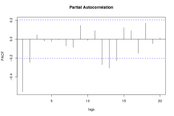
Title produced by software

(Partial) Autocorrelation Function

Date of computation

Wed, 05 Dec 2007 07:15:29 -0700

Cite this page as follows

Statistical Computations at FreeStatistics.org, Office for Research Development and Education, URL https://freestatistics.org/blog/index.php?v=date/2007/Dec/05/t1196863481jy4fm062gqkwt7a.htm/, Retrieved Fri, 03 May 2024 03:09:46 +0000

Statistical Computations at FreeStatistics.org, Office for Research Development and Education, URL https://freestatistics.org/blog/index.php?pk=2475, Retrieved Fri, 03 May 2024 03:09:46 +0000

QR Codes:

Paste this QR Code to cite your computation.

Original text written by user:

IsPrivate?

No (this computation is public)

User-defined keywords

bridome

Estimated Impact

245

Family? (F = Feedback message, R = changed R code, M = changed R Module, P = changed Parameters, D = changed Data)

-       [(Partial) Autocorrelation Function] [workshop3 correla...] [2007-12-05 14:15:29] [ff60737d3854dcb913eacf6907ce202b] [Current]

Feedback Forum

Post a new message

Dataseries X:

Download CSV

Histogram

Boxplots

Summary of compuational transaction
Raw Input	view raw input (R code)
Raw Output	view raw output of R engine
Computing time	1 seconds
R Server	'Gwilym Jenkins' @ 72.249.127.135

\begin{tabular}{lllllllll}
\hline
Summary of compuational transaction \tabularnewline
Raw Input & view raw input (R code)  \tabularnewline
Raw Output & view raw output of R engine  \tabularnewline
Computing time & 1 seconds \tabularnewline
R Server & 'Gwilym Jenkins' @ 72.249.127.135 \tabularnewline
\hline
\end{tabular}
%Source: https://freestatistics.org/blog/index.php?pk=2475&T=0

[TABLE]
[ROW][C]Summary of compuational transaction[/C][/ROW]
[ROW][C]Raw Input[/C][C]view raw input (R code) [/C][/ROW]
[ROW][C]Raw Output[/C][C]view raw output of R engine [/C][/ROW]
[ROW][C]Computing time[/C][C]1 seconds[/C][/ROW]
[ROW][C]R Server[/C][C]'Gwilym Jenkins' @ 72.249.127.135[/C][/ROW]
[/TABLE]
Source: https://freestatistics.org/blog/index.php?pk=2475&T=0

Globally Unique Identifier (entire table): ba.freestatistics.org/blog/index.php?pk=2475&T=0

As an alternative you can also use a QR Code:

The GUIDs for individual cells are displayed in the table below:

Summary of compuational transaction
Raw Input	view raw input (R code)
Raw Output	view raw output of R engine
Computing time	1 seconds
R Server	'Gwilym Jenkins' @ 72.249.127.135

Autocorrelation Function
Time lag k	ACF(k)	T-STAT	P-value
0	1	9.6437	0
1	-0.558315	-5.3842	1
2	0.141118	1.3609	0.088418
3	0.071148	0.6861	0.247169
4	-0.119585	-1.1532	0.874116
5	0.066069	0.6371	0.262799
6	-0.01211	-0.1168	0.546359
7	-0.060329	-0.5818	0.718943
8	0.023683	0.2284	0.409924
9	0.116893	1.1273	0.131263
10	-0.173629	-1.6744	0.951296
11	0.187225	1.8055	0.037113
12	-0.289854	-2.7953	0.99685
13	0.082313	0.7938	0.214667
14	-0.001096	-0.0106	0.504206
15	0.055395	0.5342	0.297236
16	-0.075535	-0.7284	0.76591
17	-0.027206	-0.2624	0.603189
18	0.245976	2.3721	0.009874
19	-0.280252	-2.7027	0.995911

\begin{tabular}{lllllllll}
\hline
Autocorrelation Function \tabularnewline
Time lag k & ACF(k) & T-STAT & P-value \tabularnewline
0 & 1 & 9.6437 & 0 \tabularnewline
1 & -0.558315 & -5.3842 & 1 \tabularnewline
2 & 0.141118 & 1.3609 & 0.088418 \tabularnewline
3 & 0.071148 & 0.6861 & 0.247169 \tabularnewline
4 & -0.119585 & -1.1532 & 0.874116 \tabularnewline
5 & 0.066069 & 0.6371 & 0.262799 \tabularnewline
6 & -0.01211 & -0.1168 & 0.546359 \tabularnewline
7 & -0.060329 & -0.5818 & 0.718943 \tabularnewline
8 & 0.023683 & 0.2284 & 0.409924 \tabularnewline
9 & 0.116893 & 1.1273 & 0.131263 \tabularnewline
10 & -0.173629 & -1.6744 & 0.951296 \tabularnewline
11 & 0.187225 & 1.8055 & 0.037113 \tabularnewline
12 & -0.289854 & -2.7953 & 0.99685 \tabularnewline
13 & 0.082313 & 0.7938 & 0.214667 \tabularnewline
14 & -0.001096 & -0.0106 & 0.504206 \tabularnewline
15 & 0.055395 & 0.5342 & 0.297236 \tabularnewline
16 & -0.075535 & -0.7284 & 0.76591 \tabularnewline
17 & -0.027206 & -0.2624 & 0.603189 \tabularnewline
18 & 0.245976 & 2.3721 & 0.009874 \tabularnewline
19 & -0.280252 & -2.7027 & 0.995911 \tabularnewline
\hline
\end{tabular}
%Source: https://freestatistics.org/blog/index.php?pk=2475&T=1

[TABLE]
[ROW][C]Autocorrelation Function[/C][/ROW]
[ROW][C]Time lag k[/C][C]ACF(k)[/C][C]T-STAT[/C][C]P-value[/C][/ROW]
[ROW][C]0[/C][C]1[/C][C]9.6437[/C][C]0[/C][/ROW]
[ROW][C]1[/C][C]-0.558315[/C][C]-5.3842[/C][C]1[/C][/ROW]
[ROW][C]2[/C][C]0.141118[/C][C]1.3609[/C][C]0.088418[/C][/ROW]
[ROW][C]3[/C][C]0.071148[/C][C]0.6861[/C][C]0.247169[/C][/ROW]
[ROW][C]4[/C][C]-0.119585[/C][C]-1.1532[/C][C]0.874116[/C][/ROW]
[ROW][C]5[/C][C]0.066069[/C][C]0.6371[/C][C]0.262799[/C][/ROW]
[ROW][C]6[/C][C]-0.01211[/C][C]-0.1168[/C][C]0.546359[/C][/ROW]
[ROW][C]7[/C][C]-0.060329[/C][C]-0.5818[/C][C]0.718943[/C][/ROW]
[ROW][C]8[/C][C]0.023683[/C][C]0.2284[/C][C]0.409924[/C][/ROW]
[ROW][C]9[/C][C]0.116893[/C][C]1.1273[/C][C]0.131263[/C][/ROW]
[ROW][C]10[/C][C]-0.173629[/C][C]-1.6744[/C][C]0.951296[/C][/ROW]
[ROW][C]11[/C][C]0.187225[/C][C]1.8055[/C][C]0.037113[/C][/ROW]
[ROW][C]12[/C][C]-0.289854[/C][C]-2.7953[/C][C]0.99685[/C][/ROW]
[ROW][C]13[/C][C]0.082313[/C][C]0.7938[/C][C]0.214667[/C][/ROW]
[ROW][C]14[/C][C]-0.001096[/C][C]-0.0106[/C][C]0.504206[/C][/ROW]
[ROW][C]15[/C][C]0.055395[/C][C]0.5342[/C][C]0.297236[/C][/ROW]
[ROW][C]16[/C][C]-0.075535[/C][C]-0.7284[/C][C]0.76591[/C][/ROW]
[ROW][C]17[/C][C]-0.027206[/C][C]-0.2624[/C][C]0.603189[/C][/ROW]
[ROW][C]18[/C][C]0.245976[/C][C]2.3721[/C][C]0.009874[/C][/ROW]
[ROW][C]19[/C][C]-0.280252[/C][C]-2.7027[/C][C]0.995911[/C][/ROW]
[/TABLE]
Source: https://freestatistics.org/blog/index.php?pk=2475&T=1

Globally Unique Identifier (entire table): ba.freestatistics.org/blog/index.php?pk=2475&T=1

As an alternative you can also use a QR Code:

The GUIDs for individual cells are displayed in the table below:

Autocorrelation Function
Time lag k	ACF(k)	T-STAT	P-value
0	1	9.6437	0
1	-0.558315	-5.3842	1
2	0.141118	1.3609	0.088418
3	0.071148	0.6861	0.247169
4	-0.119585	-1.1532	0.874116
5	0.066069	0.6371	0.262799
6	-0.01211	-0.1168	0.546359
7	-0.060329	-0.5818	0.718943
8	0.023683	0.2284	0.409924
9	0.116893	1.1273	0.131263
10	-0.173629	-1.6744	0.951296
11	0.187225	1.8055	0.037113
12	-0.289854	-2.7953	0.99685
13	0.082313	0.7938	0.214667
14	-0.001096	-0.0106	0.504206
15	0.055395	0.5342	0.297236
16	-0.075535	-0.7284	0.76591
17	-0.027206	-0.2624	0.603189
18	0.245976	2.3721	0.009874
19	-0.280252	-2.7027	0.995911

Partial Autocorrelation Function
Time lag k	PACF(k)	T-STAT	P-value
0	-0.558315	-5.3842	1
1	-0.24786	-2.3903	0.990574
2	0.048113	0.464	0.32187
3	-0.021342	-0.2058	0.581308
4	-0.026024	-0.251	0.598803
5	-0.006149	-0.0593	0.52358
6	-0.073225	-0.7062	0.759071
7	-0.087786	-0.8466	0.800299
8	0.145748	1.4055	0.081596
9	-0.013096	-0.1263	0.550113
10	0.090578	0.8735	0.19232
11	-0.270677	-2.6103	0.994728
12	-0.307992	-2.9702	0.998107
13	-0.229623	-2.2144	0.985378
14	0.122622	1.1825	0.120006
15	0.090749	0.8752	0.191873
16	-0.150504	-1.4514	0.924984
17	0.171552	1.6544	0.05071
18	-0.048067	-0.4635	0.677971
19	0.013382	0.1291	0.448798

\begin{tabular}{lllllllll}
\hline
Partial Autocorrelation Function \tabularnewline
Time lag k & PACF(k) & T-STAT & P-value \tabularnewline
0 & -0.558315 & -5.3842 & 1 \tabularnewline
1 & -0.24786 & -2.3903 & 0.990574 \tabularnewline
2 & 0.048113 & 0.464 & 0.32187 \tabularnewline
3 & -0.021342 & -0.2058 & 0.581308 \tabularnewline
4 & -0.026024 & -0.251 & 0.598803 \tabularnewline
5 & -0.006149 & -0.0593 & 0.52358 \tabularnewline
6 & -0.073225 & -0.7062 & 0.759071 \tabularnewline
7 & -0.087786 & -0.8466 & 0.800299 \tabularnewline
8 & 0.145748 & 1.4055 & 0.081596 \tabularnewline
9 & -0.013096 & -0.1263 & 0.550113 \tabularnewline
10 & 0.090578 & 0.8735 & 0.19232 \tabularnewline
11 & -0.270677 & -2.6103 & 0.994728 \tabularnewline
12 & -0.307992 & -2.9702 & 0.998107 \tabularnewline
13 & -0.229623 & -2.2144 & 0.985378 \tabularnewline
14 & 0.122622 & 1.1825 & 0.120006 \tabularnewline
15 & 0.090749 & 0.8752 & 0.191873 \tabularnewline
16 & -0.150504 & -1.4514 & 0.924984 \tabularnewline
17 & 0.171552 & 1.6544 & 0.05071 \tabularnewline
18 & -0.048067 & -0.4635 & 0.677971 \tabularnewline
19 & 0.013382 & 0.1291 & 0.448798 \tabularnewline
\hline
\end{tabular}
%Source: https://freestatistics.org/blog/index.php?pk=2475&T=2

[TABLE]
[ROW][C]Partial Autocorrelation Function[/C][/ROW]
[ROW][C]Time lag k[/C][C]PACF(k)[/C][C]T-STAT[/C][C]P-value[/C][/ROW]
[ROW][C]0[/C][C]-0.558315[/C][C]-5.3842[/C][C]1[/C][/ROW]
[ROW][C]1[/C][C]-0.24786[/C][C]-2.3903[/C][C]0.990574[/C][/ROW]
[ROW][C]2[/C][C]0.048113[/C][C]0.464[/C][C]0.32187[/C][/ROW]
[ROW][C]3[/C][C]-0.021342[/C][C]-0.2058[/C][C]0.581308[/C][/ROW]
[ROW][C]4[/C][C]-0.026024[/C][C]-0.251[/C][C]0.598803[/C][/ROW]
[ROW][C]5[/C][C]-0.006149[/C][C]-0.0593[/C][C]0.52358[/C][/ROW]
[ROW][C]6[/C][C]-0.073225[/C][C]-0.7062[/C][C]0.759071[/C][/ROW]
[ROW][C]7[/C][C]-0.087786[/C][C]-0.8466[/C][C]0.800299[/C][/ROW]
[ROW][C]8[/C][C]0.145748[/C][C]1.4055[/C][C]0.081596[/C][/ROW]
[ROW][C]9[/C][C]-0.013096[/C][C]-0.1263[/C][C]0.550113[/C][/ROW]
[ROW][C]10[/C][C]0.090578[/C][C]0.8735[/C][C]0.19232[/C][/ROW]
[ROW][C]11[/C][C]-0.270677[/C][C]-2.6103[/C][C]0.994728[/C][/ROW]
[ROW][C]12[/C][C]-0.307992[/C][C]-2.9702[/C][C]0.998107[/C][/ROW]
[ROW][C]13[/C][C]-0.229623[/C][C]-2.2144[/C][C]0.985378[/C][/ROW]
[ROW][C]14[/C][C]0.122622[/C][C]1.1825[/C][C]0.120006[/C][/ROW]
[ROW][C]15[/C][C]0.090749[/C][C]0.8752[/C][C]0.191873[/C][/ROW]
[ROW][C]16[/C][C]-0.150504[/C][C]-1.4514[/C][C]0.924984[/C][/ROW]
[ROW][C]17[/C][C]0.171552[/C][C]1.6544[/C][C]0.05071[/C][/ROW]
[ROW][C]18[/C][C]-0.048067[/C][C]-0.4635[/C][C]0.677971[/C][/ROW]
[ROW][C]19[/C][C]0.013382[/C][C]0.1291[/C][C]0.448798[/C][/ROW]
[/TABLE]
Source: https://freestatistics.org/blog/index.php?pk=2475&T=2

Globally Unique Identifier (entire table): ba.freestatistics.org/blog/index.php?pk=2475&T=2

As an alternative you can also use a QR Code:

The GUIDs for individual cells are displayed in the table below:

Partial Autocorrelation Function
Time lag k	PACF(k)	T-STAT	P-value
0	-0.558315	-5.3842	1
1	-0.24786	-2.3903	0.990574
2	0.048113	0.464	0.32187
3	-0.021342	-0.2058	0.581308
4	-0.026024	-0.251	0.598803
5	-0.006149	-0.0593	0.52358
6	-0.073225	-0.7062	0.759071
7	-0.087786	-0.8466	0.800299
8	0.145748	1.4055	0.081596
9	-0.013096	-0.1263	0.550113
10	0.090578	0.8735	0.19232
11	-0.270677	-2.6103	0.994728
12	-0.307992	-2.9702	0.998107
13	-0.229623	-2.2144	0.985378
14	0.122622	1.1825	0.120006
15	0.090749	0.8752	0.191873
16	-0.150504	-1.4514	0.924984
17	0.171552	1.6544	0.05071
18	-0.048067	-0.4635	0.677971
19	0.013382	0.1291	0.448798

Figure 1

PNG link

Postscript link

PDF link

Figure 2

PNG link

Postscript link

PDF link

Parameters (Session):

par1 = Default ; par2 = 1 ; par3 = 1 ; par4 = 1 ; par5 = 12 ;

Parameters (R input):

par1 = Default ; par2 = 1 ; par3 = 1 ; par4 = 1 ; par5 = 12 ;

R code (references can be found in the software module):

if (par1 == 'Default') {
par1 = 10*log10(length(x))
} else {
par1 <- as.numeric(par1)
}
par2 <- as.numeric(par2)
par3 <- as.numeric(par3)
par4 <- as.numeric(par4)
par5 <- as.numeric(par5)
if (par2 == 0) {
x <- log(x)
} else {
x <- (x ^ par2 - 1) / par2
}
if (par3 > 0) x <- diff(x,lag=1,difference=par3)
if (par4 > 0) x <- diff(x,lag=par5,difference=par4)
bitmap(file='pic1.png')
racf <- acf(x,par1,main='Autocorrelation',xlab='lags',ylab='ACF')
dev.off()
bitmap(file='pic2.png')
rpacf <- pacf(x,par1,main='Partial Autocorrelation',xlab='lags',ylab='PACF')
dev.off()
(myacf <- c(racf$acf))
(mypacf <- c(rpacf$acf))
lengthx <- length(x)
sqrtn <- sqrt(lengthx)
load(file='createtable')
a<-table.start()
a<-table.row.start(a)
a<-table.element(a,'Autocorrelation Function',4,TRUE)
a<-table.row.end(a)
a<-table.row.start(a)
a<-table.element(a,'Time lag k',header=TRUE)
a<-table.element(a,hyperlink('basics.htm','ACF(k)','click here for more information about the Autocorrelation Function'),header=TRUE)
a<-table.element(a,'T-STAT',header=TRUE)
a<-table.element(a,'P-value',header=TRUE)
a<-table.row.end(a)
for (i in 1:par1) {
a<-table.row.start(a)
a<-table.element(a,i-1,header=TRUE)
a<-table.element(a,round(myacf[i],6))
mytstat <- myacf[i]*sqrtn
a<-table.element(a,round(mytstat,4))
a<-table.element(a,round(1-pt(mytstat,lengthx),6))
a<-table.row.end(a)
}
a<-table.end(a)
table.save(a,file='mytable.tab')
a<-table.start()
a<-table.row.start(a)
a<-table.element(a,'Partial Autocorrelation Function',4,TRUE)
a<-table.row.end(a)
a<-table.row.start(a)
a<-table.element(a,'Time lag k',header=TRUE)
a<-table.element(a,hyperlink('basics.htm','PACF(k)','click here for more information about the Partial Autocorrelation Function'),header=TRUE)
a<-table.element(a,'T-STAT',header=TRUE)
a<-table.element(a,'P-value',header=TRUE)
a<-table.row.end(a)
for (i in 1:par1) {
a<-table.row.start(a)
a<-table.element(a,i-1,header=TRUE)
a<-table.element(a,round(mypacf[i],6))
mytstat <- mypacf[i]*sqrtn
a<-table.element(a,round(mytstat,4))
a<-table.element(a,round(1-pt(mytstat,lengthx),6))
a<-table.row.end(a)
}
a<-table.end(a)
table.save(a,file='mytable1.tab')

Free Statistics

Description of Statistical Computation

Tree of Dependent Computations

Dataset

Tables (Output of Computation)

Figures (Output of Computation)

Input Parameters & R Code