Multiple Lineair Regression

*The author of this computation has been verified*

R Software Module: /rwasp_multipleregression.wasp (opens new window with default values)

Title produced by software: Multiple Regression

Date of computation: Mon, 22 Nov 2010 17:37:46 +0000

Cite this page as follows:

Statistical Computations at FreeStatistics.org, Office for Research Development and Education, URL http://www.freestatistics.org/blog/date/2010/Nov/22/t1290447413tuo5acpe19u37eb.htm/, Retrieved Mon, 22 Nov 2010 18:37:05 +0100

BibTeX entries for LaTeX users:

@Manual{KEY, author = {{YOUR NAME}}, publisher = {Office for Research Development and Education}, title = {Statistical Computations at FreeStatistics.org, URL http://www.freestatistics.org/blog/date/2010/Nov/22/t1290447413tuo5acpe19u37eb.htm/}, year = {2010}, } @Manual{R, title = {R: A Language and Environment for Statistical Computing}, author = {{R Development Core Team}}, organization = {R Foundation for Statistical Computing}, address = {Vienna, Austria}, year = {2010}, note = {{ISBN} 3-900051-07-0}, url = {http://www.R-project.org}, }

Original text written by user:

IsPrivate?

No (this computation is public)

User-defined keywords:

Dataseries X:

» Textbox « » Textfile « » CSV «

13 13 0 14 0 13 0 3 0 12 12 12 8 8 13 13 5 5 15 10 10 12 12 16 16 6 6 12 9 9 7 7 12 12 6 6 10 10 0 10 0 11 0 5 0 12 12 0 7 0 12 0 3 0 15 13 13 16 16 18 18 8 8 9 12 12 11 11 11 11 4 4 12 12 12 14 14 14 14 4 4 11 6 6 6 6 9 9 4 4 11 5 0 16 0 14 0 6 0 11 12 12 11 11 12 12 6 6 15 11 11 16 16 11 11 5 5 7 14 0 12 0 12 0 4 0 11 14 0 7 0 13 0 6 0 11 12 12 13 13 11 11 4 4 10 12 12 11 11 12 12 6 6 14 11 0 15 0 16 0 6 0 10 11 11 7 7 9 9 4 4 6 7 0 9 0 11 0 4 0 11 9 9 7 7 13 13 2 2 15 11 0 14 0 15 0 7 0 11 11 11 15 15 10 10 5 5 12 12 0 7 0 11 0 4 0 14 12 12 15 15 13 13 6 6 15 11 0 17 0 16 0 6 0 9 11 0 15 0 15 0 7 0 13 8 8 14 14 14 14 5 5 13 9 0 14 0 14 0 6 0 16 12 12 8 8 14 14 4 4 13 10 10 8 8 8 8 4 4 12 10 0 14 0 13 0 7 0 14 12 12 14 14 15 15 7 7 11 8 0 8 0 13 0 4 0 9 12 12 11 11 11 11 4 4 16 11 0 16 0 15 0 6 0 12 12 12 10 10 15 15 6 6 10 7 0 8 0 9 0 5 0 13 11 11 14 14 13 13 6 6 16 11 11 16 16 16 16 7 7 14 12 0 13 0 13 0 6 0 15 9 9 5 5 11 11 3 3 5 15 15 8 8 12 12 3 3 8 11 0 10 0 etc...

Output produced by software:

Enter (or paste) a matrix (table) containing all data (time) series. Every column represents a different variable and must be delimited by a space or Tab. Every row represents a period in time (or category) and must be delimited by hard returns. The easiest way to enter data is to copy and paste a block of spreadsheet cells. Please, do not use commas or spaces to seperate groups of digits! Summary of computational transaction Raw Input view raw input (R code) Raw Output view raw output of R engine Computing time 10 seconds R Server 'Gwilym Jenkins' @ 72.249.127.135 Multiple Linear Regression - Estimated Regression Equation Popularity[t] = + 0.303717782313307 + 0.176147992195911FindingFriends[t] -0.151288107973995`Findingfriends*G`[t] + 0.240478962981778KnowingPeople[t] + 0.0325063503433276`Knowingpeople*G`[t] + 0.215766283815847Liked[t] + 0.219515353217923`Liked*G`[t] + 0.708072246853356Celebrity[t] -0.166549255423799`Celebrity*G`[t] + e[t] Multiple Linear Regression - Ordinary Least Squares Variable Parameter S.D. T-STAT H0: parameter = 0 2-tail p-value 1-tail p-value (Intercept) 0.303717782313307 1.415616 0.2145 0.830417 0.415208 FindingFriends 0.176147992195911 0.114094 1.5439 0.124765 0.062383 `Findingfriends*G` -0.151288107973995 0.142194 -1.064 0.289092 0.144546 KnowingPeople 0.240478962981778 0.110803 2.1703 0.031588 0.015794 `Knowingpeople*G` 0.0325063503433276 0.133519 0.2435 0.807989 0.403994 Liked 0.215766283815847 0.14089 1.5315 0.127806 0.063903 `Liked*G` 0.219515353217923 0.174534 1.2577 0.210487 0.105243 Celebrity 0.708072246853356 0.292824 2.4181 0.016826 0.008413 `Celebrity*G` -0.166549255423799 0.345665 -0.4818 0.630648 0.315324 Multiple Linear Regression - Regression Statistics Multiple R 0.721556275076144 R-squared 0.52064345810176 Adjusted R-squared 0.494556027250155 F-TEST (value) 19.9576363446204 F-TEST (DF numerator) 8 F-TEST (DF denominator) 147 p-value 0 Multiple Linear Regression - Residual Statistics Residual Standard Deviation 2.0877829424917 Sum Squared Residuals 640.749129399017 Multiple Linear Regression - Actuals, Interpolation, and Residuals Time or Index Actuals Interpolation Forecast Residuals Prediction Error 1 13 10.8895255927711 2.11047440722889 2 12 11.1521951381639 0.847804861836061 3 15 14.0417845255514 0.958215474448622 4 12 10.9108715265689 1.08912847343113 5 10 10.3837776903313 -0.383777690331296 6 12 8.81425857588693 3.18574142411307 7 15 17.1619146884442 -2.16191468844422 8 9 10.5590648126422 -1.55906481264216 9 12 12.6838656637188 -0.683865663718782 10 11 8.1744156666176 2.82558433338241 11 11 12.3012826055433 -1.30128260554330 12 11 12.0773924325350 -1.07739243253504 13 15 12.4406544864753 2.55934551352468 14 7 11.0770216220410 -4.07702162204099 15 11 11.5065375846547 -0.506537584654662 16 11 11.1050354392924 -0.105035439292366 17 10 12.0773924325350 -2.07739243253504 18 14 13.5492241633687 0.450775836631309 19 10 8.57170040105228 1.42829959894772 20 6 8.90678250390843 -2.90678250390843 21 11 9.18006119788441 1.81993880211559 22 15 13.8010511634244 1.19894883657558 23 11 11.7323875361164 -0.732387536116447 24 12 9.30656453892443 2.69343546107557 25 14 13.6046153228692 0.39538467713077 26 15 14.0301820893322 0.969817910667754 27 9 14.0415301264062 -5.0415301264062 28 13 13.1259491182607 -0.125949118260674 29 13 12.5249166483634 0.475083351636604 30 16 11.0459537837681 4.95404621623185 31 13 8.3845441931217 4.6154558068783 32 12 13.1933706035968 -1.19337060359682 33 14 14.7437162750412 -0.743716275041222 34 11 9.27398410075426 1.72601589924574 35 9 10.5590648126422 -1.55906481264216 36 16 13.5739368425346 2.42606315746538 37 12 13.1102520303112 -1.11025203031124 38 10 8.94284322014831 1.05715677985169 39 13 13.3067701253222 -0.306770125322209 40 16 15.7001086545033 0.299891345496714 41 14 12.5971153781535 1.40288462184649 42 15 8.30505028859622 6.69494971140378 43 5 9.7084471709368 -4.7084471709368 44 8 10.0676197194897 -2.0676197194897 45 11 11.2335766083378 -0.233576608337807 46 16 13.3448059166268 2.65519408337320 47 17 13.4735140842515 3.52648591574847 48 9 8.94723070108285 0.0527692989171527 49 9 12.2192765072424 -3.21927650724244 50 13 15.1834455472956 -2.18344554729565 51 10 10.8747621896182 -0.874762189618176 52 6 12.1180967598976 -6.11809675989763 53 12 11.8643304521342 0.135669547865782 54 8 9.9785760695379 -1.97857606953790 55 14 12.0651911234961 1.93480887650394 56 12 12.7652471338927 -0.765247133892652 57 11 11.1927521103353 -0.192752110335282 58 16 15.1088658946299 0.891134105370103 59 8 9.29877407723053 -1.29877407723053 60 15 15.5333646955740 -0.533364695573968 61 7 9.0547375388687 -2.0547375388687 62 16 13.5343185509147 2.46568144908531 63 14 14.1866952864701 -0.186695286470134 64 16 14.1773333993897 1.82266660061025 65 9 10.0963632218142 -1.09636322181421 66 14 12.5171217047895 1.48287829521054 67 11 12.8623070203012 -1.86230702030121 68 13 10.2304030695936 2.76959693040637 69 15 13.0586446962190 1.94135530378098 70 5 6.22668143776913 -1.22668143776913 71 15 12.7652471338927 2.23475286610735 72 13 12.5171217047895 0.482878295210537 73 11 11.4477034969565 -0.447703496956529 74 11 12.6437715232232 -1.64377152322320 75 12 12.7359396144501 -0.735939614450082 76 12 13.6046153228692 -1.60461532286923 77 12 12.3796852653027 -0.379685265302714 78 12 12.4176821679018 -0.417682167901798 79 14 11.0459537837681 2.95404621623185 80 6 8.11109226315751 -2.11109226315751 81 7 9.52233082274028 -2.52233082274028 82 14 12.4742037538538 1.52579624614625 83 14 14.3396297230984 -0.339629723098414 84 10 11.4861496726617 -1.48614967266165 85 13 8.33330064992337 4.66669935007663 86 12 12.3170181235518 -0.317018123551792 87 9 9.15512922589445 -0.155129225894450 88 12 12.7174149310972 -0.717414931097212 89 16 15.2603793822489 0.739620617751137 90 10 9.82714075650792 0.172859243492077 91 14 13.5206737831231 0.479326216876903 92 10 13.9043480860646 -3.90434808606464 93 16 15.7249685387252 0.275031461274797 94 15 13.8278808677505 1.17211913224950 95 12 11.0161709293248 0.983829070675166 96 10 9.74010887266684 0.259891127333161 97 8 10.4774774551835 -2.47747745518349 98 8 8.55887400045114 -0.55887400045114 99 11 11.8564626931300 -0.856462693129975 100 13 12.5126740695688 0.487325930431191 101 16 15.9730939678284 0.0269060321716083 102 16 15.0167015883663 0.983298411633672 103 14 14.9901586335517 -0.990158633551675 104 11 9.20047344688567 1.79952655311433 105 4 6.60092088806472 -2.60092088806472 106 14 14.6534395344260 -0.653439534426044 107 9 10.8383853268363 -1.83838532683631 108 14 15.5333646955740 -1.53336469557397 109 8 11.0006816505450 -3.00068165054497 110 8 11.6299213130174 -3.62992131301744 111 11 12.6296982600543 -1.62969826005430 112 12 14.0466987774111 -2.04669877741112 113 11 11.4207328162684 -0.420732816268387 114 14 13.9292079702866 0.0707920297134405 115 15 13.7120075134726 1.28799248652737 116 16 13.7420517623560 2.25794823764402 117 16 13.7669116465779 2.23308835342210 118 11 12.0420194146922 -1.04201941469216 119 14 13.2938395879329 0.706160412067092 120 14 10.5485776454533 3.45142235454674 121 12 11.7026134000348 0.297386599965199 122 14 12.2185657442337 1.78143425576628 123 8 9.82714075650792 -1.82714075650792 124 13 13.4699875801288 -0.46998758012882 125 16 13.2938395879329 2.70616041206709 126 12 11.0415061485475 0.958493851452505 127 16 15.7205209035045 0.279479096495450 128 12 13.6046153228692 -1.60461532286923 129 11 12.0340078649603 -1.03400786496025 130 4 6.04772724989257 -2.04772724989257 131 16 15.7205209035045 0.279479096495450 132 15 12.760799498672 2.239200501328 133 10 11.9165170578357 -1.91651705783569 134 13 13.4080972278583 -0.408097227858265 135 15 12.8128816619694 2.18711833803065 136 12 10.8836574600595 1.11634253994052 137 14 13.117691595737 0.882308404263004 138 7 10.9987940848966 -3.99879408489658 139 19 14.4751785969368 4.52482140306323 140 12 13.1756688867045 -1.17566888670451 141 12 11.7262597811962 0.273740218803786 142 13 13.0533606249511 -0.0533606249511303 143 15 13.5544289377863 1.44557106221368 144 8 8.59687402439871 -0.596874024398706 145 12 11.1566427733846 0.84335722661541 146 10 10.6266367605150 -0.626636760514988 147 8 10.9024146002071 -2.90241460020711 148 10 14.0380498483365 -4.03804984833649 149 15 13.3581705587188 1.64182944128123 150 16 14.7392686398206 1.26073136017943 151 13 13.3023224901016 -0.302322490101555 152 16 15.4519832254001 0.548016774599902 153 9 10.4235159388038 -1.42351593880380 154 14 12.4358729984116 1.5641270015884 155 14 12.4456800651235 1.55431993487648 156 12 10.7570038566624 1.24299614333756 Goldfeld-Quandt test for Heteroskedasticity p-values Alternative Hypothesis breakpoint index greater 2-sided less 12 0.0148846440769442 0.0297692881538884 0.985115355923056 13 0.270367171934365 0.54073434386873 0.729632828065635 14 0.452738580422579 0.905477160845158 0.547261419577421 15 0.389044558071467 0.778089116142934 0.610955441928533 16 0.276315944135212 0.552631888270424 0.723684055864788 17 0.235200479882294 0.470400959764589 0.764799520117706 18 0.204340223034756 0.408680446069512 0.795659776965244 19 0.173504075125319 0.347008150250639 0.82649592487468 20 0.592540890119907 0.814918219760185 0.407459109880093 21 0.514915020553154 0.970169958893693 0.485084979446846 22 0.628094801832265 0.74381039633547 0.371905198167735 23 0.55325496882702 0.89349006234596 0.44674503117298 24 0.535315395432962 0.929369209134076 0.464684604567038 25 0.468126579253763 0.936253158507525 0.531873420746237 26 0.450052518477259 0.900105036954519 0.549947481522741 27 0.572164399366448 0.855671201267104 0.427835600633552 28 0.515245281531433 0.969509436937133 0.484754718468567 29 0.47256789059977 0.94513578119954 0.52743210940023 30 0.656623223302466 0.686753553395067 0.343376776697534 31 0.791957586015767 0.416084827968467 0.208042413984233 32 0.769104639811598 0.461790720376803 0.230895360188402 33 0.72016070876808 0.55967858246384 0.27983929123192 34 0.682663579072978 0.634672841854044 0.317336420927022 35 0.685076429537626 0.629847140924748 0.314923570462374 36 0.745622651723302 0.508754696553397 0.254377348276698 37 0.720143966453238 0.559712067093523 0.279856033546762 38 0.679312296762485 0.64137540647503 0.320687703237515 39 0.625390911420816 0.749218177158368 0.374609088579184 40 0.580955240167808 0.838089519664383 0.419044759832192 41 0.57615307976735 0.8476938404653 0.42384692023265 42 0.836294121196182 0.327411757607635 0.163705878803818 43 0.944939600945146 0.110120798109708 0.0550603990548541 44 0.954875370139415 0.0902492597211698 0.0451246298605849 45 0.94223098825242 0.115538023495162 0.0577690117475809 46 0.95981750997817 0.0803649800436617 0.0401824900218309 47 0.97438791061741 0.0512241787651819 0.0256120893825910 48 0.96617470249647 0.0676505950070607 0.0338252975035304 49 0.979247374158265 0.0415052516834708 0.0207526258417354 50 0.979779674816592 0.0404406503668161 0.0202203251834080 51 0.974027405471502 0.051945189056996 0.025972594528498 52 0.996860285932767 0.00627942813446516 0.00313971406723258 53 0.995429796880836 0.00914040623832878 0.00457020311916439 54 0.996502020401508 0.0069959591969838 0.0034979795984919 55 0.996628550692515 0.00674289861497084 0.00337144930748542 56 0.99539510372897 0.00920979254206052 0.00460489627103026 57 0.993843588774736 0.0123128224505288 0.00615641122526438 58 0.991733896728822 0.0165322065423565 0.00826610327117827 59 0.991759954653213 0.0164800906935736 0.00824004534678678 60 0.98881901924196 0.0223619615160791 0.0111809807580395 61 0.9893008756718 0.0213982486563988 0.0106991243281994 62 0.99162227861669 0.016755442766622 0.008377721383311 63 0.988439811817906 0.0231203763641873 0.0115601881820937 64 0.987275009119605 0.0254499817607891 0.0127249908803945 65 0.985464003473448 0.0290719930531038 0.0145359965265519 66 0.983124120031612 0.0337517599367754 0.0168758799683877 67 0.982730008719138 0.0345399825617251 0.0172699912808625 68 0.986243887365243 0.0275122252695143 0.0137561126347572 69 0.986093386505474 0.0278132269890531 0.0139066134945265 70 0.983264873700425 0.033470252599149 0.0167351262995745 71 0.983952833005262 0.0320943339894756 0.0160471669947378 72 0.978743511892171 0.0425129762156572 0.0212564881078286 73 0.972155674548958 0.0556886509020846 0.0278443254510423 74 0.970049565314358 0.0599008693712843 0.0299504346856422 75 0.96216949605184 0.0756610078963196 0.0378305039481598 76 0.95795278436673 0.0840944312665404 0.0420472156332702 77 0.947008750444686 0.105982499110627 0.0529912495553137 78 0.935509515496803 0.128980969006394 0.0644904845031971 79 0.949698181643263 0.100603636713475 0.0503018183567374 80 0.952358834397114 0.0952823312057727 0.0476411656028863 81 0.956683961435184 0.086632077129632 0.043316038564816 82 0.956439291433866 0.0871214171322678 0.0435607085661339 83 0.944775217018713 0.110449565962575 0.0552247829812873 84 0.937492091445042 0.125015817109916 0.0625079085549582 85 0.990164132554969 0.0196717348900629 0.00983586744503145 86 0.98691637540894 0.02616724918212 0.01308362459106 87 0.982929157927117 0.034141684145766 0.017070842072883 88 0.98011878313635 0.0397624337273017 0.0198812168636508 89 0.974653369327958 0.0506932613440848 0.0253466306720424 90 0.969186284745768 0.0616274305084647 0.0308137152542324 91 0.961437358968518 0.0771252820629644 0.0385626410314822 92 0.982707754985226 0.0345844900295482 0.0172922450147741 93 0.976696160274005 0.0466076794519893 0.0233038397259947 94 0.972235967753082 0.0555280644938356 0.0277640322469178 95 0.966669858890535 0.0666602822189292 0.0333301411094646 96 0.956037744874722 0.0879245102505565 0.0439622551252783 97 0.95414638268592 0.0917072346281603 0.0458536173140801 98 0.951585182800178 0.0968296343996447 0.0484148171998223 99 0.949950511715705 0.100098976568590 0.0500494882842949 100 0.935840018472108 0.128319963055784 0.0641599815278922 101 0.91772783289984 0.164544334200320 0.0822721671001602 102 0.901372102246794 0.197255795506412 0.0986278977532062 103 0.900379568307531 0.199240863384939 0.0996204316924694 104 0.913638471767218 0.172723056465563 0.0863615282327816 105 0.92160393619139 0.156792127617220 0.0783960638086098 106 0.905080534980456 0.189838930039087 0.0949194650195436 107 0.894429209817369 0.211141580365262 0.105570790182631 108 0.889313923951246 0.221372152097508 0.110686076048754 109 0.903514003491531 0.192971993016938 0.0964859965084689 110 0.930852808776104 0.138294382447791 0.0691471912238956 111 0.926802528012315 0.146394943975369 0.0731974719876846 112 0.9441847247261 0.1116305505478 0.0558152752739 113 0.92619333897152 0.147613322056960 0.0738066610284801 114 0.904464404152022 0.191071191695956 0.095535595847978 115 0.880871630988122 0.238256738023756 0.119128369011878 116 0.876708961081778 0.246582077836443 0.123291038918222 117 0.881594411496969 0.236811177006062 0.118405588503031 118 0.855064887972663 0.289870224054673 0.144935112027337 119 0.820592561253514 0.358814877492971 0.179407438746486 120 0.941442736498356 0.117114527003287 0.0585572635016436 121 0.92237837011889 0.155243259762219 0.0776216298811095 122 0.903788175871854 0.192423648256292 0.096211824128146 123 0.888066944665287 0.223866110669425 0.111933055334713 124 0.855615312362776 0.288769375274448 0.144384687637224 125 0.854742073912206 0.290515852175588 0.145257926087794 126 0.825531619683513 0.348936760632973 0.174468380316487 127 0.779937688607489 0.440124622785022 0.220062311392511 128 0.771910269209207 0.456179461581585 0.228089730790793 129 0.774090906217091 0.451818187565818 0.225909093782909 130 0.733977715527072 0.532044568945855 0.266022284472928 131 0.685945193791664 0.628109612416673 0.314054806208336 132 0.664865901028745 0.670268197942509 0.335134098971255 133 0.765809370205923 0.468381259588155 0.234190629794077 134 0.70446240082087 0.591075198358260 0.295537599179130 135 0.736481317349152 0.527037365301696 0.263518682650848 136 0.701595930249042 0.596808139501917 0.298404069750958 137 0.622107042530114 0.755785914939772 0.377892957469886 138 0.746905905494873 0.506188189010254 0.253094094505127 139 0.96208041821085 0.0758391635783024 0.0379195817891512 140 0.991564584116266 0.0168708317674676 0.0084354158837338 141 0.987862844543467 0.0242743109130662 0.0121371554565331 142 0.967172934632297 0.0656541307354055 0.0328270653677028 143 0.918753170800533 0.162493658398933 0.0812468291994665 144 0.833472140086662 0.333055719826677 0.166527859913338 Meta Analysis of Goldfeld-Quandt test for Heteroskedasticity Description # significant tests % significant tests OK/NOK 1% type I error level 5 0.037593984962406 NOK 5% type I error level 32 0.240601503759398 NOK 10% type I error level 54 0.406015037593985 NOK

Charts produced by software:

http://www.freestatistics.org/blog/date/2010/Nov/22/t1290447413tuo5acpe19u37eb/10kl1t1290447455.png (open in new window) http://www.freestatistics.org/blog/date/2010/Nov/22/t1290447413tuo5acpe19u37eb/10kl1t1290447455.ps (open in new window) http://www.freestatistics.org/blog/date/2010/Nov/22/t1290447413tuo5acpe19u37eb/1dk4h1290447455.png (open in new window) http://www.freestatistics.org/blog/date/2010/Nov/22/t1290447413tuo5acpe19u37eb/1dk4h1290447455.ps (open in new window) http://www.freestatistics.org/blog/date/2010/Nov/22/t1290447413tuo5acpe19u37eb/26b321290447455.png (open in new window) http://www.freestatistics.org/blog/date/2010/Nov/22/t1290447413tuo5acpe19u37eb/26b321290447455.ps (open in new window) http://www.freestatistics.org/blog/date/2010/Nov/22/t1290447413tuo5acpe19u37eb/36b321290447455.png (open in new window) http://www.freestatistics.org/blog/date/2010/Nov/22/t1290447413tuo5acpe19u37eb/36b321290447455.ps (open in new window) http://www.freestatistics.org/blog/date/2010/Nov/22/t1290447413tuo5acpe19u37eb/46b321290447455.png (open in new window) http://www.freestatistics.org/blog/date/2010/Nov/22/t1290447413tuo5acpe19u37eb/46b321290447455.ps (open in new window) http://www.freestatistics.org/blog/date/2010/Nov/22/t1290447413tuo5acpe19u37eb/5z3l51290447455.png (open in new window) http://www.freestatistics.org/blog/date/2010/Nov/22/t1290447413tuo5acpe19u37eb/5z3l51290447455.ps (open in new window) http://www.freestatistics.org/blog/date/2010/Nov/22/t1290447413tuo5acpe19u37eb/6z3l51290447455.png (open in new window) http://www.freestatistics.org/blog/date/2010/Nov/22/t1290447413tuo5acpe19u37eb/6z3l51290447455.ps (open in new window) http://www.freestatistics.org/blog/date/2010/Nov/22/t1290447413tuo5acpe19u37eb/7rckq1290447455.png (open in new window) http://www.freestatistics.org/blog/date/2010/Nov/22/t1290447413tuo5acpe19u37eb/7rckq1290447455.ps (open in new window) http://www.freestatistics.org/blog/date/2010/Nov/22/t1290447413tuo5acpe19u37eb/8rckq1290447455.png (open in new window) http://www.freestatistics.org/blog/date/2010/Nov/22/t1290447413tuo5acpe19u37eb/8rckq1290447455.ps (open in new window) http://www.freestatistics.org/blog/date/2010/Nov/22/t1290447413tuo5acpe19u37eb/9kl1t1290447455.png (open in new window) http://www.freestatistics.org/blog/date/2010/Nov/22/t1290447413tuo5acpe19u37eb/9kl1t1290447455.ps (open in new window)

Parameters (Session):

par1 = 1 ; par2 = Do not include Seasonal Dummies ; par3 = No Linear Trend ;

Parameters (R input):

par1 = 1 ; par2 = Do not include Seasonal Dummies ; par3 = No Linear Trend ;

R code (references can be found in the software module):

library(lattice) library(lmtest) n25 <- 25 #minimum number of obs. for Goldfeld-Quandt test par1 <- as.numeric(par1) x <- t(y) k <- length(x[1,]) n <- length(x[,1]) x1 <- cbind(x[,par1], x[,1:k!=par1]) mycolnames <- c(colnames(x)[par1], colnames(x)[1:k!=par1]) colnames(x1) <- mycolnames #colnames(x)[par1] x <- x1 if (par3 == 'First Differences'){ x2 <- array(0, dim=c(n-1,k), dimnames=list(1:(n-1), paste('(1-B)',colnames(x),sep=''))) for (i in 1:n-1) { for (j in 1:k) { x2[i,j] <- x[i+1,j] - x[i,j] } } x <- x2 } if (par2 == 'Include Monthly Dummies'){ x2 <- array(0, dim=c(n,11), dimnames=list(1:n, paste('M', seq(1:11), sep =''))) for (i in 1:11){ x2[seq(i,n,12),i] <- 1 } x <- cbind(x, x2) } if (par2 == 'Include Quarterly Dummies'){ x2 <- array(0, dim=c(n,3), dimnames=list(1:n, paste('Q', seq(1:3), sep =''))) for (i in 1:3){ x2[seq(i,n,4),i] <- 1 } x <- cbind(x, x2) } k <- length(x[1,]) if (par3 == 'Linear Trend'){ x <- cbind(x, c(1:n)) colnames(x)[k+1] <- 't' } x k <- length(x[1,]) df <- as.data.frame(x) (mylm <- lm(df)) (mysum <- summary(mylm)) if (n > n25) { kp3 <- k + 3 nmkm3 <- n - k - 3 gqarr <- array(NA, dim=c(nmkm3-kp3+1,3)) numgqtests <- 0 numsignificant1 <- 0 numsignificant5 <- 0 numsignificant10 <- 0 for (mypoint in kp3:nmkm3) { j <- 0 numgqtests <- numgqtests + 1 for (myalt in c('greater', 'two.sided', 'less')) { j <- j + 1 gqarr[mypoint-kp3+1,j] <- gqtest(mylm, point=mypoint, alternative=myalt)$p.value } if (gqarr[mypoint-kp3+1,2] < 0.01) numsignificant1 <- numsignificant1 + 1 if (gqarr[mypoint-kp3+1,2] < 0.05) numsignificant5 <- numsignificant5 + 1 if (gqarr[mypoint-kp3+1,2] < 0.10) numsignificant10 <- numsignificant10 + 1 } gqarr } bitmap(file='test0.png') plot(x[,1], type='l', main='Actuals and Interpolation', ylab='value of Actuals and Interpolation (dots)', xlab='time or index') points(x[,1]-mysum$resid) grid() dev.off() bitmap(file='test1.png') plot(mysum$resid, type='b', pch=19, main='Residuals', ylab='value of Residuals', xlab='time or index') grid() dev.off() bitmap(file='test2.png') hist(mysum$resid, main='Residual Histogram', xlab='values of Residuals') grid() dev.off() bitmap(file='test3.png') 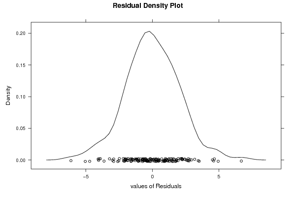densityplot(~mysum$resid,col='black',main='Residual Density Plot', xlab='values of Residuals') dev.off() bitmap(file='test4.png') 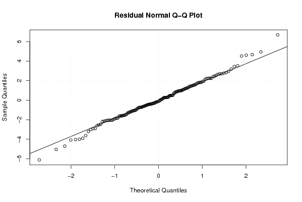qqnorm(mysum$resid, main='Residual Normal Q-Q Plot') qqline(mysum$resid) grid() dev.off() (myerror <- as.ts(mysum$resid)) bitmap(file='test5.png') 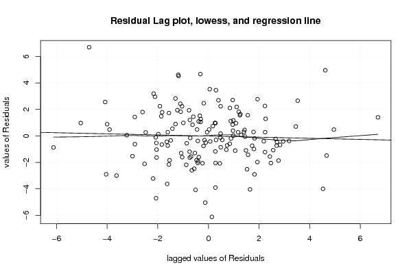dum <- cbind(lag(myerror,k=1),myerror) dum dum1 <- dum[2:length(myerror),] dum1 z <- as.data.frame(dum1) z plot(z,main=paste('Residual Lag plot, lowess, and regression line'), ylab='values of Residuals', xlab='lagged values of Residuals') lines(lowess(z)) abline(lm(z)) grid() dev.off() bitmap(file='test6.png') 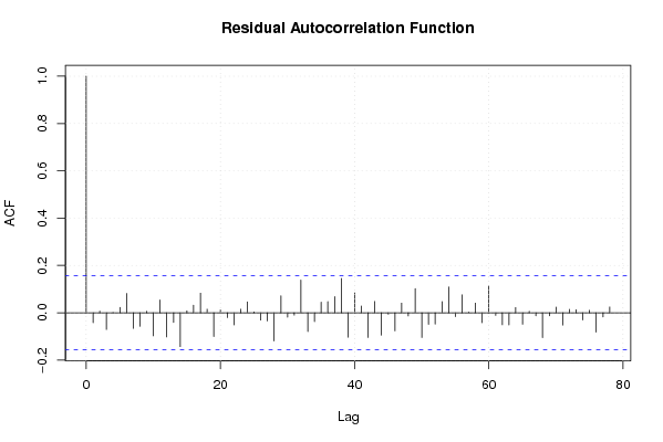acf(mysum$resid, lag.max=length(mysum$resid)/2, main='Residual Autocorrelation Function') grid() dev.off() bitmap(file='test7.png') 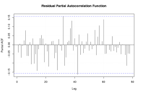pacf(mysum$resid, lag.max=length(mysum$resid)/2, main='Residual Partial Autocorrelation Function') grid() dev.off() bitmap(file='test8.png') 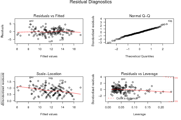opar <- par(mfrow = c(2,2), oma = c(0, 0, 1.1, 0)) plot(mylm, las = 1, sub='Residual Diagnostics') par(opar) dev.off() if (n > n25) { bitmap(file='test9.png') plot(kp3:nmkm3,gqarr[,2], main='Goldfeld-Quandt test',ylab='2-sided p-value',xlab='breakpoint') grid() dev.off() } load(file='createtable') a<-table.start() a<-table.row.start(a) a<-table.element(a, 'Multiple Linear Regression - Estimated Regression Equation', 1, TRUE) a<-table.row.end(a) myeq <- colnames(x)[1] myeq <- paste(myeq, '[t] = ', sep='') for (i in 1:k){ if (mysum$coefficients[i,1] > 0) myeq <- paste(myeq, '+', '') myeq <- paste(myeq, mysum$coefficients[i,1], sep=' ') if (rownames(mysum$coefficients)[i] != '(Intercept)') { myeq <- paste(myeq, rownames(mysum$coefficients)[i], sep='') if (rownames(mysum$coefficients)[i] != 't') myeq <- paste(myeq, '[t]', sep='') } } myeq <- paste(myeq, ' + e[t]') a<-table.row.start(a) a<-table.element(a, myeq) a<-table.row.end(a) a<-table.end(a) table.save(a,file='mytable1.tab') a<-table.start() a<-table.row.start(a) a<-table.element(a,hyperlink('http://www.xycoon.com/ols1.htm','Multiple Linear Regression - Ordinary Least Squares',''), 6, TRUE) a<-table.row.end(a) a<-table.row.start(a) a<-table.element(a,'Variable',header=TRUE) a<-table.element(a,'Parameter',header=TRUE) a<-table.element(a,'S.D.',header=TRUE) a<-table.element(a,'T-STAT<br />H0: parameter = 0',header=TRUE) a<-table.element(a,'2-tail p-value',header=TRUE) a<-table.element(a,'1-tail p-value',header=TRUE) a<-table.row.end(a) for (i in 1:k){ a<-table.row.start(a) a<-table.element(a,rownames(mysum$coefficients)[i],header=TRUE) a<-table.element(a,mysum$coefficients[i,1]) a<-table.element(a, round(mysum$coefficients[i,2],6)) a<-table.element(a, round(mysum$coefficients[i,3],4)) a<-table.element(a, round(mysum$coefficients[i,4],6)) a<-table.element(a, round(mysum$coefficients[i,4]/2,6)) a<-table.row.end(a) } a<-table.end(a) table.save(a,file='mytable2.tab') a<-table.start() a<-table.row.start(a) a<-table.element(a, 'Multiple Linear Regression - Regression Statistics', 2, TRUE) a<-table.row.end(a) a<-table.row.start(a) a<-table.element(a, 'Multiple R',1,TRUE) a<-table.element(a, sqrt(mysum$r.squared)) a<-table.row.end(a) a<-table.row.start(a) a<-table.element(a, 'R-squared',1,TRUE) a<-table.element(a, mysum$r.squared) a<-table.row.end(a) a<-table.row.start(a) a<-table.element(a, 'Adjusted R-squared',1,TRUE) a<-table.element(a, mysum$adj.r.squared) a<-table.row.end(a) a<-table.row.start(a) a<-table.element(a, 'F-TEST (value)',1,TRUE) a<-table.element(a, mysum$fstatistic[1]) a<-table.row.end(a) a<-table.row.start(a) a<-table.element(a, 'F-TEST (DF numerator)',1,TRUE) a<-table.element(a, mysum$fstatistic[2]) a<-table.row.end(a) a<-table.row.start(a) a<-table.element(a, 'F-TEST (DF denominator)',1,TRUE) a<-table.element(a, mysum$fstatistic[3]) a<-table.row.end(a) a<-table.row.start(a) a<-table.element(a, 'p-value',1,TRUE) a<-table.element(a, 1-pf(mysum$fstatistic[1],mysum$fstatistic[2],mysum$fstatistic[3])) a<-table.row.end(a) a<-table.row.start(a) a<-table.element(a, 'Multiple Linear Regression - Residual Statistics', 2, TRUE) a<-table.row.end(a) a<-table.row.start(a) a<-table.element(a, 'Residual Standard Deviation',1,TRUE) a<-table.element(a, mysum$sigma) a<-table.row.end(a) a<-table.row.start(a) a<-table.element(a, 'Sum Squared Residuals',1,TRUE) a<-table.element(a, sum(myerror*myerror)) a<-table.row.end(a) a<-table.end(a) table.save(a,file='mytable3.tab') a<-table.start() a<-table.row.start(a) a<-table.element(a, 'Multiple Linear Regression - Actuals, Interpolation, and Residuals', 4, TRUE) a<-table.row.end(a) a<-table.row.start(a) a<-table.element(a, 'Time or Index', 1, TRUE) a<-table.element(a, 'Actuals', 1, TRUE) a<-table.element(a, 'Interpolation<br />Forecast', 1, TRUE) a<-table.element(a, 'Residuals<br />Prediction Error', 1, TRUE) a<-table.row.end(a) for (i in 1:n) { a<-table.row.start(a) a<-table.element(a,i, 1, TRUE) a<-table.element(a,x[i]) a<-table.element(a,x[i]-mysum$resid[i]) a<-table.element(a,mysum$resid[i]) a<-table.row.end(a) } a<-table.end(a) table.save(a,file='mytable4.tab') if (n > n25) { a<-table.start() a<-table.row.start(a) a<-table.element(a,'Goldfeld-Quandt test for Heteroskedasticity',4,TRUE) a<-table.row.end(a) a<-table.row.start(a) a<-table.element(a,'p-values',header=TRUE) a<-table.element(a,'Alternative Hypothesis',3,header=TRUE) a<-table.row.end(a) a<-table.row.start(a) a<-table.element(a,'breakpoint index',header=TRUE) a<-table.element(a,'greater',header=TRUE) a<-table.element(a,'2-sided',header=TRUE) a<-table.element(a,'less',header=TRUE) a<-table.row.end(a) for (mypoint in kp3:nmkm3) { a<-table.row.start(a) a<-table.element(a,mypoint,header=TRUE) a<-table.element(a,gqarr[mypoint-kp3+1,1]) a<-table.element(a,gqarr[mypoint-kp3+1,2]) a<-table.element(a,gqarr[mypoint-kp3+1,3]) a<-table.row.end(a) } a<-table.end(a) table.save(a,file='mytable5.tab') a<-table.start() a<-table.row.start(a) a<-table.element(a,'Meta Analysis of Goldfeld-Quandt test for Heteroskedasticity',4,TRUE) a<-table.row.end(a) a<-table.row.start(a) a<-table.element(a,'Description',header=TRUE) a<-table.element(a,'# significant tests',header=TRUE) a<-table.element(a,'% significant tests',header=TRUE) a<-table.element(a,'OK/NOK',header=TRUE) a<-table.row.end(a) a<-table.row.start(a) a<-table.element(a,'1% type I error level',header=TRUE) a<-table.element(a,numsignificant1) a<-table.element(a,numsignificant1/numgqtests) if (numsignificant1/numgqtests < 0.01) dum <- 'OK' else dum <- 'NOK' a<-table.element(a,dum) a<-table.row.end(a) a<-table.row.start(a) a<-table.element(a,'5% type I error level',header=TRUE) a<-table.element(a,numsignificant5) a<-table.element(a,numsignificant5/numgqtests) if (numsignificant5/numgqtests < 0.05) dum <- 'OK' else dum <- 'NOK' a<-table.element(a,dum) a<-table.row.end(a) a<-table.row.start(a) a<-table.element(a,'10% type I error level',header=TRUE) a<-table.element(a,numsignificant10) a<-table.element(a,numsignificant10/numgqtests) if (numsignificant10/numgqtests < 0.1) dum <- 'OK' else dum <- 'NOK' a<-table.element(a,dum) a<-table.row.end(a) a<-table.end(a) table.save(a,file='mytable6.tab') }

Copyright

This work is licensed under a Creative Commons Attribution-Noncommercial-Share Alike 3.0 License.

Software written by Ed van Stee & Patrick Wessa

Disclaimer

Information provided on this web site is provided "AS IS" without warranty of any kind, either express or implied, including, without limitation, warranties of merchantability, fitness for a particular purpose, and noninfringement. We use reasonable efforts to include accurate and timely information and periodically update the information, and software without notice. However, we make no warranties or representations as to the accuracy or completeness of such information (or software), and we assume no liability or responsibility for errors or omissions in the content of this web site, or any software bugs in online applications. Your use of this web site is AT YOUR OWN RISK. Under no circumstances and under no legal theory shall we be liable to you or any other person for any direct, indirect, special, incidental, exemplary, or consequential damages arising from your access to, or use of, this web site.

Privacy Policy

We may request personal information to be submitted to our servers in order to be able to:

• personalize online software applications according to your needs
• enforce strict security rules with respect to the data that you upload (e.g. statistical data)
• manage user sessions of online applications
• alert you about important changes or upgrades in resources or applications

We NEVER allow other companies to directly offer registered users information about their products and services. Banner references and hyperlinks of third parties NEVER contain any personal data of the visitor.

We do NOT sell, nor transmit by any means, personal information, nor statistical data series uploaded by you to third parties.

We carefully protect your data from loss, misuse, alteration, and destruction. However, at any time, and under any circumstance you are solely responsible for managing your passwords, and keeping them secret.

We store a unique ANONYMOUS USER ID in the form of a small 'Cookie' on your computer. This allows us to track your progress when using this website which is necessary to create state-dependent features. The cookie is used for NO OTHER PURPOSE. At any time you may opt to disallow cookies from this website - this will not affect other features of this website.

We examine cookies that are used by third-parties (banner and online ads) very closely: abuse from third-parties automatically results in termination of the advertising contract without refund. We have very good reason to believe that the cookies that are produced by third parties (banner ads) do NOT cause any privacy or security risk.

FreeStatistics.org is safe. There is no need to download any software to use the applications and services contained in this website. Hence, your system's security is not compromised by their use, and your personal data - other than data you submit in the account application form, and the user-agent information that is transmitted by your browser - is never transmitted to our servers.

As a general rule, we do not log on-line behavior of individuals (other than normal logging of webserver 'hits'). However, in cases of abuse, hacking, unauthorized access, Denial of Service attacks, illegal copying, hotlinking, non-compliance with international webstandards (such as robots.txt), or any other harmful behavior, our system engineers are empowered to log, track, identify, publish, and ban misbehaving individuals - even if this leads to ban entire blocks of IP addresses, or disclosing user's identity.

FreeStatistics.org is powered by