Home » date » 2010 » Dec » 24 »

workshop 10 - multiple regression 2 (jonas poels)

*Unverified author*

R Software Module: /rwasp_multipleregression.wasp (opens new window with default values)

Title produced by software: Multiple Regression

Date of computation: Fri, 24 Dec 2010 20:00:47 +0000

Cite this page as follows:

Statistical Computations at FreeStatistics.org, Office for Research Development and Education, URL http://www.freestatistics.org/blog/date/2010/Dec/24/t1293220715embaqwpkn2j5w8g.htm/, Retrieved Fri, 24 Dec 2010 20:58:46 +0100

BibTeX entries for LaTeX users:

@Manual{KEY,
    author = {{YOUR NAME}},
    publisher = {Office for Research Development and Education},
    title = {Statistical Computations at FreeStatistics.org, URL http://www.freestatistics.org/blog/date/2010/Dec/24/t1293220715embaqwpkn2j5w8g.htm/},
    year = {2010},
}
@Manual{R,
    title = {R: A Language and Environment for Statistical Computing},
    author = {{R Development Core Team}},
    organization = {R Foundation for Statistical Computing},
    address = {Vienna, Austria},
    year = {2010},
    note = {{ISBN} 3-900051-07-0},
    url = {http://www.R-project.org},
}

Original text written by user:

IsPrivate?

No (this computation is public)

User-defined keywords:

Dataseries X:

» Textbox « » Textfile « » CSV «

1 162556 162556 1081 1081 213118 213118 230380558 6282929 1 29790 29790 309 309 81767 81767 25266003 4324047 1 87550 87550 458 458 153198 153198 70164684 4108272 0 84738 0 588 0 -26007 0 -15292116 -1212617 1 54660 54660 299 299 126942 126942 37955658 1485329 1 42634 42634 156 156 157214 157214 24525384 1779876 0 40949 0 481 0 129352 0 62218312 1367203 1 42312 42312 323 323 234817 234817 75845891 2519076 1 37704 37704 452 452 60448 60448 27322496 912684 1 16275 16275 109 109 47818 47818 5212162 1443586 0 25830 0 115 0 245546 0 28237790 1220017 0 12679 0 110 0 48020 0 5282200 984885 1 18014 18014 239 239 -1710 -1710 -408690 1457425 0 43556 0 247 0 32648 0 8064056 -572920 1 24524 24524 497 497 95350 95350 47388950 929144 0 6532 0 103 0 151352 0 15589256 1151176 0 7123 0 109 0 288170 0 31410530 790090 1 20813 20813 502 502 114337 114337 57397174 774497 1 37597 37597 248 248 37884 37884 9395232 990576 0 17821 0 373 0 122844 0 45820812 454195 1 12988 12988 119 119 82340 82340 9798460 876607 1 2 etc...

Output produced by software:

Enter (or paste) a matrix (table) containing all data (time) series. Every column represents a different variable and must be delimited by a space or Tab. Every row represents a period in time (or category) and must be delimited by hard returns. The easiest way to enter data is to copy and paste a block of spreadsheet cells. Please, do not use commas or spaces to seperate groups of digits!

Summary of computational transaction
Raw Input	view raw input (R code)
Raw Output	view raw output of R engine
Computing time	8 seconds
R Server	'Gwilym Jenkins' @ 72.249.127.135
R Framework error message	The field 'Names of X columns' contains a hard return which cannot be interpreted. Please, resubmit your request without hard returns in the 'Names of X columns'.

Multiple Linear Regression - Estimated Regression Equation

Trades[t] = + 78.1233889151631 + 85.2298042625602Group[t] + 0.00528577879449569Costs[t] -0.00724477872667004GrCosts[t] + 0.327954919331716GrTrades[t] -0.000616431833275788Dividends[t] -0.000603374741996059GrDiv[t] + 6.4698704385376e-06TrDiv[t] -2.22387688513800e-05`Wealth `[t] + e[t]

Multiple Linear Regression - Ordinary Least Squares
Variable	Parameter	S.D.	T-STAT H0: parameter = 0	2-tail p-value	1-tail p-value
(Intercept)	78.1233889151631	19.818065	3.942	0.000158	7.9e-05
Group	85.2298042625602	32.765553	2.6012	0.010842	0.005421
Costs	0.00528577879449569	0.000682	7.7537	0	0
GrCosts	-0.00724477872667004	0.001195	-6.0616	0	0
GrTrades	0.327954919331716	0.111126	2.9512	0.004025	0.002013
Dividends	-0.000616431833275788	0.000174	-3.5368	0.00064	0.00032
GrDiv	-0.000603374741996059	0.00027	-2.2346	0.027891	0.013946
TrDiv	6.4698704385376e-06	0	15.0288	0	0
`Wealth `	-2.22387688513800e-05	1.6e-05	-1.4021	0.164291	0.082146

Multiple Linear Regression - Regression Statistics
Multiple R	0.943928684452234
R-squared	0.891001361331725
Adjusted R-squared	0.881419063426821
F-TEST (value)	92.9841015353732
F-TEST (DF numerator)	8
F-TEST (DF denominator)	91
p-value	0
Multiple Linear Regression - Residual Statistics
Residual Standard Deviation	65.3720585028906
Sum Squared Residuals	388889.048994387

Multiple Linear Regression - Actuals, Interpolation, and Residuals
Time or Index	Actuals	Interpolation Forecast	Residuals Prediction Error
1	1081	1290.27028636935	-209.270286369352
2	309	173.899015205695	135.100984794305
3	458	317.767677905623	140.232322094377
4	588	470.090355008308	117.909644991692
5	299	212.024392857289	86.975607142711
6	156	58.3172925476256	97.6827074523744
7	481	586.973560327673	-105.973560327673
8	323	334.654045588482	-11.6540455884825
9	452	320.467856078033	131.532143921967
10	109	110.507282145974	-1.50728214597428
11	115	218.855850956329	-103.855850956329
12	110	127.813241386923	-17.8132413869226
13	239	173.475354320781	65.524645679219
14	247	353.139936574874	-106.139936574874
15	497	447.933064869461	49.0669351305388
16	103	94.6116347527906	8.3883652472094
17	109	123.788260497284	-14.7882604972836
18	502	501.873292256154	0.126707743845785
19	248	163.579083510709	84.4209164892912
20	373	382.950280095076	-9.95028009507616
21	119	120.397570301925	-1.39757030192455
22	84	77.3512183752393	6.64878162476068
23	102	140.142112888261	-38.1421128882605
24	295	308.20291248134	-13.20291248134
25	105	114.318357057162	-9.31835705716223
26	64	136.814711895112	-72.8147118951122
27	267	224.786787818827	42.2132121811726
28	129	145.598837131620	-16.5988371316204
29	37	93.8632556984867	-56.8632556984867
30	361	229.643412627325	131.356587372675
31	28	60.0886728337764	-32.0886728337764
32	85	83.4637922517271	1.53620774827286
33	44	73.985100389802	-29.985100389802
34	49	65.075765960423	-16.0757659604230
35	22	-71.4365888993478	93.4365888993478
36	155	207.366775271174	-52.366775271174
37	91	115.760059262576	-24.7600592625762
38	81	85.6981675956595	-4.69816759565952
39	79	33.1427357339363	45.8572642660637
40	145	120.27846975875	24.7215302412499
41	816	709.35486565987	106.645134340129
42	61	120.934205009002	-59.9342050090021
43	226	170.225634317545	55.7743656824548
44	105	112.622812730485	-7.62281273048548
45	62	79.2492093584405	-17.2492093584405
46	24	48.2292704057255	-24.2292704057255
47	26	-66.1901747822921	92.1901747822921
48	322	361.876651483944	-39.8766514839444
49	84	84.7010142592245	-0.701014259224468
50	33	54.6983263857004	-21.6983263857004
51	108	123.717365927723	-15.7173659277228
52	150	159.432764558925	-9.43276455892495
53	115	85.3495542356503	29.6504457643497
54	162	177.062227422668	-15.0622274226677
55	158	167.781153272940	-9.78115327294048
56	97	81.9956200032153	15.0043799967847
57	9	58.4946446940818	-49.4946446940818
58	66	79.7591185240336	-13.7591185240336
59	107	84.28249209369	22.7175079063101
60	101	119.658847553364	-18.6588475533643
61	47	70.489441278293	-23.489441278293
62	38	58.6643022000376	-20.6643022000376
63	34	64.4822914162119	-30.4822914162119
64	84	113.316261112867	-29.3162611128673
65	79	78.0079518371803	0.992048162819682
66	947	640.664891184525	306.335108815475
67	74	66.4144837751272	7.58551622487278
68	53	79.5727920153672	-26.5727920153672
69	94	74.5527650554496	19.4472349445504
70	63	85.3552983743526	-22.3552983743526
71	58	147.82577782258	-89.8257778225801
72	49	85.074898008531	-36.074898008531
73	34	36.048086352312	-2.04808635231198
74	11	30.5210151045620	-19.5210151045620
75	35	33.6116641291416	1.38833587085842
76	17	73.9533962531998	-56.9533962531998
77	47	39.3917024688289	7.60829753117108
78	43	51.3834912301866	-8.3834912301866
79	117	86.5185764155848	30.4814235844152
80	171	195.406722982970	-24.4067229829696
81	26	50.394293315634	-24.394293315634
82	73	101.290463778903	-28.2904637789025
83	59	40.8206338137077	18.1793661862923
84	18	55.9990365477834	-37.9990365477834
85	15	18.2179956274575	-3.2179956274575
86	72	119.435705834532	-47.4357058345324
87	86	81.7634174329314	4.23658256706862
88	14	17.672737828793	-3.67273782879301
89	64	59.662173037211	4.33782696278901
90	11	15.7065614138648	-4.70656141386482
91	52	53.2160822530349	-1.21608225303492
92	41	83.5888709445375	-42.5888709445375
93	99	82.0374861617833	16.9625138382167
94	75	73.7124336542594	1.28756634574059
95	45	67.9252426984615	-22.9252426984615
96	43	106.365773262194	-63.3657732621936
97	8	5.36090881999485	2.63909118000515
98	198	221.700858048041	-23.7008580480413
99	22	20.2762254808698	1.72377451913021
100	11	72.8277982265484	-61.8277982265484

Goldfeld-Quandt test for Heteroskedasticity
p-values	Alternative Hypothesis
breakpoint index	greater	2-sided	less
12	0.979808233829525	0.0403835323409503	0.0201917661704752
13	0.976391701173017	0.0472165976539669	0.0236082988269834
14	0.993705912745403	0.0125881745091932	0.00629408725459662
15	0.988693594714023	0.0226128105719538	0.0113064052859769
16	0.99125969422017	0.0174806115596603	0.00874030577983015
17	0.993466078657568	0.0130678426848632	0.00653392134243162
18	0.988352251007858	0.0232954979842851	0.0116477489921425
19	0.982581331837414	0.0348373363251728	0.0174186681625864
20	0.99931522148556	0.00136955702888155	0.000684778514440774
21	0.99917947458775	0.00164105082450064	0.00082052541225032
22	0.998858485589271	0.00228302882145740	0.00114151441072870
23	0.998693404613162	0.00261319077367653	0.00130659538683827
24	0.999285702838523	0.00142859432295326	0.000714297161476629
25	0.998823547244298	0.00235290551140371	0.00117645275570186
26	0.999606120470922	0.000787759058156866	0.000393879529078433
27	0.999515530411367	0.000968939177266244	0.000484469588633122
28	0.999155106632751	0.00168978673449848	0.00084489336724924
29	0.999337609019365	0.00132478196126967	0.000662390980634836
30	0.999999808923266	3.82153467491008e-07	1.91076733745504e-07
31	0.999999788750192	4.22499615528942e-07	2.11249807764471e-07
32	0.999999583777843	8.32444313281477e-07	4.16222156640738e-07
33	0.999999347209253	1.30558149371287e-06	6.52790746856435e-07
34	0.999998724527354	2.55094529172982e-06	1.27547264586491e-06
35	0.999998768021437	2.46395712633943e-06	1.23197856316971e-06
36	0.999998519494113	2.96101177393364e-06	1.48050588696682e-06
37	0.9999978527853	4.29442939773425e-06	2.14721469886712e-06
38	0.999995592643544	8.81471291282235e-06	4.40735645641117e-06
39	0.999991370974873	1.72580502530967e-05	8.62902512654836e-06
40	0.999988352830332	2.32943393357603e-05	1.16471696678801e-05
41	1	2.54216742961474e-18	1.27108371480737e-18
42	1	7.04715505132021e-18	3.52357752566011e-18
43	1	1.86449673819117e-17	9.32248369095586e-18
44	1	4.57567080334027e-17	2.28783540167013e-17
45	1	1.82320327419440e-16	9.11601637097198e-17
46	1	5.48494250336775e-16	2.74247125168387e-16
47	1	3.75168034923947e-18	1.87584017461974e-18
48	1	5.88955466364779e-22	2.94477733182389e-22
49	1	1.70943239505903e-21	8.54716197529514e-22
50	1	9.29738785925414e-21	4.64869392962707e-21
51	1	3.95141716336058e-20	1.97570858168029e-20
52	1	1.46796460524443e-19	7.33982302622213e-20
53	1	7.96042500215624e-19	3.98021250107812e-19
54	1	6.3855021447219e-19	3.19275107236095e-19
55	1	8.68193618839187e-21	4.34096809419593e-21
56	1	1.89861880478230e-20	9.49309402391152e-21
57	1	1.16303126846672e-20	5.81515634233361e-21
58	1	5.72659775415654e-20	2.86329887707827e-20
59	1	3.47332210650841e-19	1.73666105325420e-19
60	1	1.64317190818739e-18	8.21585954093697e-19
61	1	9.2730289474471e-18	4.63651447372355e-18
62	1	5.78597861869941e-17	2.89298930934970e-17
63	1	2.34500331631749e-16	1.17250165815874e-16
64	1	1.20533254120017e-15	6.02666270600085e-16
65	0.999999999999997	5.39879383429415e-15	2.69939691714708e-15
66	1	8.53302296221315e-17	4.26651148110657e-17
67	1	3.28936922103785e-16	1.64468461051892e-16
68	1	1.48816856894878e-15	7.44084284474388e-16
69	0.999999999999999	2.8988026447174e-15	1.4494013223587e-15
70	0.99999999999999	1.85009889097916e-14	9.2504944548958e-15
71	0.999999999999984	3.23797725845355e-14	1.61898862922677e-14
72	0.999999999999886	2.28883131998517e-13	1.14441565999259e-13
73	0.999999999999136	1.72739385143351e-12	8.63696925716754e-13
74	0.999999999994233	1.15340758578255e-11	5.76703792891275e-12
75	0.999999999958839	8.23224688240744e-11	4.11612344120372e-11
76	0.999999999834363	3.31273600297376e-10	1.65636800148688e-10
77	0.999999998864592	2.27081545449372e-09	1.13540772724686e-09
78	0.999999993046206	1.39075889303011e-08	6.95379446515056e-09
79	0.999999996612856	6.77428710985091e-09	3.38714355492546e-09
80	0.999999999896356	2.07288961910417e-10	1.03644480955208e-10
81	0.999999998964677	2.07064693810410e-09	1.03532346905205e-09
82	0.999999993823592	1.23528157509785e-08	6.17640787548927e-09
83	0.999999961283603	7.74327948802938e-08	3.87163974401469e-08
84	0.999999829394168	3.41211664880158e-07	1.70605832440079e-07
85	0.999997951397374	4.09720525191670e-06	2.04860262595835e-06
86	0.999985482730692	2.90345386153239e-05	1.45172693076619e-05
87	0.999975944182165	4.81116356692249e-05	2.40558178346124e-05
88	0.999825464148158	0.000349071703684207	0.000174535851842103

Meta Analysis of Goldfeld-Quandt test for Heteroskedasticity
Description	# significant tests	% significant tests	OK/NOK
1% type I error level	69	0.896103896103896	NOK
5% type I error level	77	1	NOK
10% type I error level	77	1	NOK

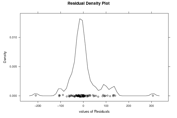
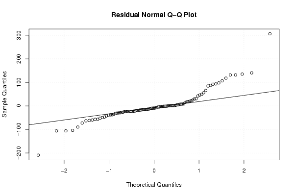
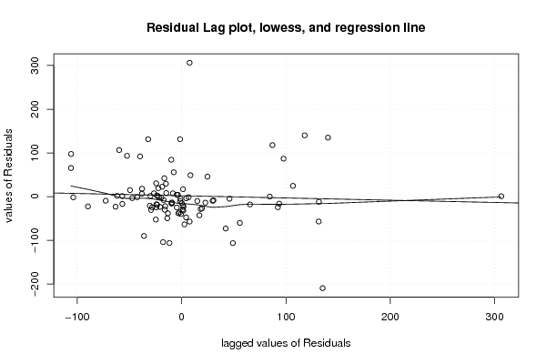
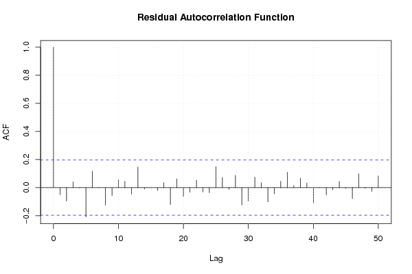
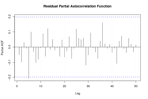
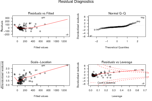
Charts produced by software:

http://www.freestatistics.org/blog/date/2010/Dec/24/t1293220715embaqwpkn2j5w8g/109eih1293220838.png (open in new window)

http://www.freestatistics.org/blog/date/2010/Dec/24/t1293220715embaqwpkn2j5w8g/109eih1293220838.ps (open in new window)

http://www.freestatistics.org/blog/date/2010/Dec/24/t1293220715embaqwpkn2j5w8g/13v361293220838.png (open in new window)

http://www.freestatistics.org/blog/date/2010/Dec/24/t1293220715embaqwpkn2j5w8g/13v361293220838.ps (open in new window)

http://www.freestatistics.org/blog/date/2010/Dec/24/t1293220715embaqwpkn2j5w8g/23v361293220838.png (open in new window)

http://www.freestatistics.org/blog/date/2010/Dec/24/t1293220715embaqwpkn2j5w8g/23v361293220838.ps (open in new window)

http://www.freestatistics.org/blog/date/2010/Dec/24/t1293220715embaqwpkn2j5w8g/3dmkr1293220838.png (open in new window)

http://www.freestatistics.org/blog/date/2010/Dec/24/t1293220715embaqwpkn2j5w8g/3dmkr1293220838.ps (open in new window)

http://www.freestatistics.org/blog/date/2010/Dec/24/t1293220715embaqwpkn2j5w8g/4dmkr1293220838.png (open in new window)

http://www.freestatistics.org/blog/date/2010/Dec/24/t1293220715embaqwpkn2j5w8g/4dmkr1293220838.ps (open in new window)

http://www.freestatistics.org/blog/date/2010/Dec/24/t1293220715embaqwpkn2j5w8g/5dmkr1293220838.png (open in new window)

http://www.freestatistics.org/blog/date/2010/Dec/24/t1293220715embaqwpkn2j5w8g/5dmkr1293220838.ps (open in new window)

http://www.freestatistics.org/blog/date/2010/Dec/24/t1293220715embaqwpkn2j5w8g/6oekc1293220838.png (open in new window)

http://www.freestatistics.org/blog/date/2010/Dec/24/t1293220715embaqwpkn2j5w8g/6oekc1293220838.ps (open in new window)

http://www.freestatistics.org/blog/date/2010/Dec/24/t1293220715embaqwpkn2j5w8g/7oekc1293220838.png (open in new window)

http://www.freestatistics.org/blog/date/2010/Dec/24/t1293220715embaqwpkn2j5w8g/7oekc1293220838.ps (open in new window)

http://www.freestatistics.org/blog/date/2010/Dec/24/t1293220715embaqwpkn2j5w8g/8z51f1293220838.png (open in new window)

http://www.freestatistics.org/blog/date/2010/Dec/24/t1293220715embaqwpkn2j5w8g/8z51f1293220838.ps (open in new window)

http://www.freestatistics.org/blog/date/2010/Dec/24/t1293220715embaqwpkn2j5w8g/9z51f1293220838.png (open in new window)

http://www.freestatistics.org/blog/date/2010/Dec/24/t1293220715embaqwpkn2j5w8g/9z51f1293220838.ps (open in new window)

Parameters (Session):

par1 = 4 ; par2 = none ; par3 = 2 ; par4 = yes ;

Parameters (R input):

par1 = 4 ; par2 = Do not include Seasonal Dummies ; par3 = No Linear Trend ; par4 = yes ;

R code (references can be found in the software module):

library(lattice)

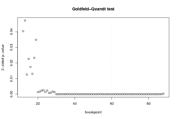
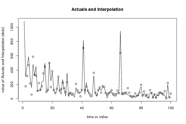
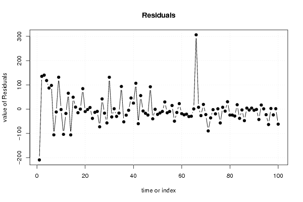
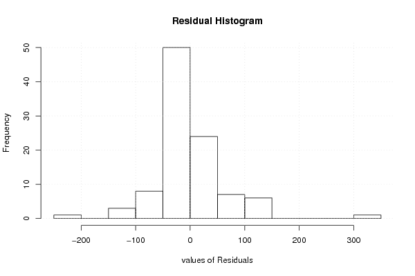
library(lmtest)

n25 <- 25 #minimum number of obs. for Goldfeld-Quandt test

par1 <- as.numeric(par1)

x <- t(y)

k <- length(x[1,])

n <- length(x[,1])

x1 <- cbind(x[,par1], x[,1:k!=par1])

mycolnames <- c(colnames(x)[par1], colnames(x)[1:k!=par1])

colnames(x1) <- mycolnames #colnames(x)[par1]

x <- x1

if (par3 == 'First Differences'){

x2 <- array(0, dim=c(n-1,k), dimnames=list(1:(n-1), paste('(1-B)',colnames(x),sep='')))

for (i in 1:n-1) {

for (j in 1:k) {

x2[i,j] <- x[i+1,j] - x[i,j]

}

}

x <- x2

}

if (par2 == 'Include Monthly Dummies'){

x2 <- array(0, dim=c(n,11), dimnames=list(1:n, paste('M', seq(1:11), sep ='')))

for (i in 1:11){

x2[seq(i,n,12),i] <- 1

}

x <- cbind(x, x2)

}

if (par2 == 'Include Quarterly Dummies'){

x2 <- array(0, dim=c(n,3), dimnames=list(1:n, paste('Q', seq(1:3), sep ='')))

for (i in 1:3){

x2[seq(i,n,4),i] <- 1

}

x <- cbind(x, x2)

}

k <- length(x[1,])

if (par3 == 'Linear Trend'){

x <- cbind(x, c(1:n))

colnames(x)[k+1] <- 't'

}

x

k <- length(x[1,])

df <- as.data.frame(x)

(mylm <- lm(df))

(mysum <- summary(mylm))

if (n > n25) {

kp3 <- k + 3

nmkm3 <- n - k - 3

gqarr <- array(NA, dim=c(nmkm3-kp3+1,3))

numgqtests <- 0

numsignificant1 <- 0

numsignificant5 <- 0

numsignificant10 <- 0

for (mypoint in kp3:nmkm3) {

j <- 0

numgqtests <- numgqtests + 1

for (myalt in c('greater', 'two.sided', 'less')) {

j <- j + 1

gqarr[mypoint-kp3+1,j] <- gqtest(mylm, point=mypoint, alternative=myalt)$p.value

}

if (gqarr[mypoint-kp3+1,2] < 0.01) numsignificant1 <- numsignificant1 + 1

if (gqarr[mypoint-kp3+1,2] < 0.05) numsignificant5 <- numsignificant5 + 1

if (gqarr[mypoint-kp3+1,2] < 0.10) numsignificant10 <- numsignificant10 + 1

}

gqarr

}

bitmap(file='test0.png')

plot(x[,1], type='l', main='Actuals and Interpolation', ylab='value of Actuals and Interpolation (dots)', xlab='time or index')

points(x[,1]-mysum$resid)

grid()

dev.off()

bitmap(file='test1.png')

plot(mysum$resid, type='b', pch=19, main='Residuals', ylab='value of Residuals', xlab='time or index')

grid()

dev.off()

bitmap(file='test2.png')

hist(mysum$resid, main='Residual Histogram', xlab='values of Residuals')

grid()

dev.off()

bitmap(file='test3.png')

densityplot(~mysum$resid,col='black',main='Residual Density Plot', xlab='values of Residuals')

dev.off()

bitmap(file='test4.png')

qqnorm(mysum$resid, main='Residual Normal Q-Q Plot')

qqline(mysum$resid)

grid()

dev.off()

(myerror <- as.ts(mysum$resid))

bitmap(file='test5.png')

dum <- cbind(lag(myerror,k=1),myerror)

dum

dum1 <- dum[2:length(myerror),]

dum1

z <- as.data.frame(dum1)

z

plot(z,main=paste('Residual Lag plot, lowess, and regression line'), ylab='values of Residuals', xlab='lagged values of Residuals')

lines(lowess(z))

abline(lm(z))

grid()

dev.off()

bitmap(file='test6.png')

acf(mysum$resid, lag.max=length(mysum$resid)/2, main='Residual Autocorrelation Function')

grid()

dev.off()

bitmap(file='test7.png')

pacf(mysum$resid, lag.max=length(mysum$resid)/2, main='Residual Partial Autocorrelation Function')

grid()

dev.off()

bitmap(file='test8.png')

opar <- par(mfrow = c(2,2), oma = c(0, 0, 1.1, 0))

plot(mylm, las = 1, sub='Residual Diagnostics')

par(opar)

dev.off()

if (n > n25) {

bitmap(file='test9.png')

plot(kp3:nmkm3,gqarr[,2], main='Goldfeld-Quandt test',ylab='2-sided p-value',xlab='breakpoint')

grid()

dev.off()

}

load(file='createtable')

a<-table.start()

a<-table.row.start(a)

a<-table.element(a, 'Multiple Linear Regression - Estimated Regression Equation', 1, TRUE)

a<-table.row.end(a)

myeq <- colnames(x)[1]

myeq <- paste(myeq, '[t] = ', sep='')

for (i in 1:k){

if (mysum$coefficients[i,1] > 0) myeq <- paste(myeq, '+', '')

myeq <- paste(myeq, mysum$coefficients[i,1], sep=' ')

if (rownames(mysum$coefficients)[i] != '(Intercept)') {

myeq <- paste(myeq, rownames(mysum$coefficients)[i], sep='')

if (rownames(mysum$coefficients)[i] != 't') myeq <- paste(myeq, '[t]', sep='')

}

}

myeq <- paste(myeq, ' + e[t]')

a<-table.row.start(a)

a<-table.element(a, myeq)

a<-table.row.end(a)

a<-table.end(a)

table.save(a,file='mytable1.tab')

a<-table.start()

a<-table.row.start(a)

a<-table.element(a,hyperlink('http://www.xycoon.com/ols1.htm','Multiple Linear Regression - Ordinary Least Squares',''), 6, TRUE)

a<-table.row.end(a)

a<-table.row.start(a)

a<-table.element(a,'Variable',header=TRUE)

a<-table.element(a,'Parameter',header=TRUE)

a<-table.element(a,'S.D.',header=TRUE)

a<-table.element(a,'T-STAT<br />H0: parameter = 0',header=TRUE)

a<-table.element(a,'2-tail p-value',header=TRUE)

a<-table.element(a,'1-tail p-value',header=TRUE)

a<-table.row.end(a)

for (i in 1:k){

a<-table.row.start(a)

a<-table.element(a,rownames(mysum$coefficients)[i],header=TRUE)

a<-table.element(a,mysum$coefficients[i,1])

a<-table.element(a, round(mysum$coefficients[i,2],6))

a<-table.element(a, round(mysum$coefficients[i,3],4))

a<-table.element(a, round(mysum$coefficients[i,4],6))

a<-table.element(a, round(mysum$coefficients[i,4]/2,6))

a<-table.row.end(a)

}

a<-table.end(a)

table.save(a,file='mytable2.tab')

a<-table.start()

a<-table.row.start(a)

a<-table.element(a, 'Multiple Linear Regression - Regression Statistics', 2, TRUE)

a<-table.row.end(a)

a<-table.row.start(a)

a<-table.element(a, 'Multiple R',1,TRUE)

a<-table.element(a, sqrt(mysum$r.squared))

a<-table.row.end(a)

a<-table.row.start(a)

a<-table.element(a, 'R-squared',1,TRUE)

a<-table.element(a, mysum$r.squared)

a<-table.row.end(a)

a<-table.row.start(a)

a<-table.element(a, 'Adjusted R-squared',1,TRUE)

a<-table.element(a, mysum$adj.r.squared)

a<-table.row.end(a)

a<-table.row.start(a)

a<-table.element(a, 'F-TEST (value)',1,TRUE)

a<-table.element(a, mysum$fstatistic[1])

a<-table.row.end(a)

a<-table.row.start(a)

a<-table.element(a, 'F-TEST (DF numerator)',1,TRUE)

a<-table.element(a, mysum$fstatistic[2])

a<-table.row.end(a)

a<-table.row.start(a)

a<-table.element(a, 'F-TEST (DF denominator)',1,TRUE)

a<-table.element(a, mysum$fstatistic[3])

a<-table.row.end(a)

a<-table.row.start(a)

a<-table.element(a, 'p-value',1,TRUE)

a<-table.element(a, 1-pf(mysum$fstatistic[1],mysum$fstatistic[2],mysum$fstatistic[3]))

a<-table.row.end(a)

a<-table.row.start(a)

a<-table.element(a, 'Multiple Linear Regression - Residual Statistics', 2, TRUE)

a<-table.row.end(a)

a<-table.row.start(a)

a<-table.element(a, 'Residual Standard Deviation',1,TRUE)

a<-table.element(a, mysum$sigma)

a<-table.row.end(a)

a<-table.row.start(a)

a<-table.element(a, 'Sum Squared Residuals',1,TRUE)

a<-table.element(a, sum(myerror*myerror))

a<-table.row.end(a)

a<-table.end(a)

table.save(a,file='mytable3.tab')

a<-table.start()

a<-table.row.start(a)

a<-table.element(a, 'Multiple Linear Regression - Actuals, Interpolation, and Residuals', 4, TRUE)

a<-table.row.end(a)

a<-table.row.start(a)

a<-table.element(a, 'Time or Index', 1, TRUE)

a<-table.element(a, 'Actuals', 1, TRUE)

a<-table.element(a, 'Interpolation<br />Forecast', 1, TRUE)

a<-table.element(a, 'Residuals<br />Prediction Error', 1, TRUE)

a<-table.row.end(a)

for (i in 1:n) {

a<-table.row.start(a)

a<-table.element(a,i, 1, TRUE)

a<-table.element(a,x[i])

a<-table.element(a,x[i]-mysum$resid[i])

a<-table.element(a,mysum$resid[i])

a<-table.row.end(a)

}

a<-table.end(a)

table.save(a,file='mytable4.tab')

if (n > n25) {

a<-table.start()

a<-table.row.start(a)

a<-table.element(a,'Goldfeld-Quandt test for Heteroskedasticity',4,TRUE)

a<-table.row.end(a)

a<-table.row.start(a)

a<-table.element(a,'p-values',header=TRUE)

a<-table.element(a,'Alternative Hypothesis',3,header=TRUE)

a<-table.row.end(a)

a<-table.row.start(a)

a<-table.element(a,'breakpoint index',header=TRUE)

a<-table.element(a,'greater',header=TRUE)

a<-table.element(a,'2-sided',header=TRUE)

a<-table.element(a,'less',header=TRUE)

a<-table.row.end(a)

for (mypoint in kp3:nmkm3) {

a<-table.row.start(a)

a<-table.element(a,mypoint,header=TRUE)

a<-table.element(a,gqarr[mypoint-kp3+1,1])

a<-table.element(a,gqarr[mypoint-kp3+1,2])

a<-table.element(a,gqarr[mypoint-kp3+1,3])

a<-table.row.end(a)

}

a<-table.end(a)

table.save(a,file='mytable5.tab')

a<-table.start()

a<-table.row.start(a)

a<-table.element(a,'Meta Analysis of Goldfeld-Quandt test for Heteroskedasticity',4,TRUE)

a<-table.row.end(a)

a<-table.row.start(a)

a<-table.element(a,'Description',header=TRUE)

a<-table.element(a,'# significant tests',header=TRUE)

a<-table.element(a,'% significant tests',header=TRUE)

a<-table.element(a,'OK/NOK',header=TRUE)

a<-table.row.end(a)

a<-table.row.start(a)

a<-table.element(a,'1% type I error level',header=TRUE)

a<-table.element(a,numsignificant1)

a<-table.element(a,numsignificant1/numgqtests)

if (numsignificant1/numgqtests < 0.01) dum <- 'OK' else dum <- 'NOK'

a<-table.element(a,dum)

a<-table.row.end(a)

a<-table.row.start(a)

a<-table.element(a,'5% type I error level',header=TRUE)

a<-table.element(a,numsignificant5)

a<-table.element(a,numsignificant5/numgqtests)

if (numsignificant5/numgqtests < 0.05) dum <- 'OK' else dum <- 'NOK'

a<-table.element(a,dum)

a<-table.row.end(a)

a<-table.row.start(a)

a<-table.element(a,'10% type I error level',header=TRUE)

a<-table.element(a,numsignificant10)

a<-table.element(a,numsignificant10/numgqtests)

if (numsignificant10/numgqtests < 0.1) dum <- 'OK' else dum <- 'NOK'

a<-table.element(a,dum)

a<-table.row.end(a)

a<-table.end(a)

table.save(a,file='mytable6.tab')

}

This work is licensed under a Creative Commons Attribution-Noncommercial-Share Alike 3.0 License.

Software written by Ed van Stee & Patrick Wessa

Disclaimer

Information provided on this web site is provided "AS IS" without warranty of any kind, either express or implied, including, without limitation, warranties of merchantability, fitness for a particular purpose, and noninfringement. We use reasonable efforts to include accurate and timely information and periodically update the information, and software without notice. However, we make no warranties or representations as to the accuracy or completeness of such information (or software), and we assume no liability or responsibility for errors or omissions in the content of this web site, or any software bugs in online applications. Your use of this web site is AT YOUR OWN RISK. Under no circumstances and under no legal theory shall we be liable to you or any other person for any direct, indirect, special, incidental, exemplary, or consequential damages arising from your access to, or use of, this web site.

We may request personal information to be submitted to our servers in order to be able to:

personalize online software applications according to your needs
enforce strict security rules with respect to the data that you upload (e.g. statistical data)
manage user sessions of online applications
alert you about important changes or upgrades in resources or applications

We NEVER allow other companies to directly offer registered users information about their products and services. Banner references and hyperlinks of third parties NEVER contain any personal data of the visitor.

We do NOT sell, nor transmit by any means, personal information, nor statistical data series uploaded by you to third parties.

We carefully protect your data from loss, misuse, alteration, and destruction. However, at any time, and under any circumstance you are solely responsible for managing your passwords, and keeping them secret.

We store a unique ANONYMOUS USER ID in the form of a small 'Cookie' on your computer. This allows us to track your progress when using this website which is necessary to create state-dependent features. The cookie is used for NO OTHER PURPOSE. At any time you may opt to disallow cookies from this website - this will not affect other features of this website.

We examine cookies that are used by third-parties (banner and online ads) very closely: abuse from third-parties automatically results in termination of the advertising contract without refund. We have very good reason to believe that the cookies that are produced by third parties (banner ads) do NOT cause any privacy or security risk.

FreeStatistics.org is safe. There is no need to download any software to use the applications and services contained in this website. Hence, your system's security is not compromised by their use, and your personal data - other than data you submit in the account application form, and the user-agent information that is transmitted by your browser - is never transmitted to our servers.

As a general rule, we do not log on-line behavior of individuals (other than normal logging of webserver 'hits'). However, in cases of abuse, hacking, unauthorized access, Denial of Service attacks, illegal copying, hotlinking, non-compliance with international webstandards (such as robots.txt), or any other harmful behavior, our system engineers are empowered to log, track, identify, publish, and ban misbehaving individuals - even if this leads to ban entire blocks of IP addresses, or disclosing user's identity.

FreeStatistics.org is powered by