Analyse temperatuur tijdreeks | |||||||||||||||||||||||||||||||||||||||||||||||||||||||||||||||||||||||||||||||||||||||||||||||||||||||||||||||||||||||||||||||||||||||||||||||||||||||||||||||||||||||||||||||||||||||||||||||||||||||||||||||||||||||||||||||||||||||||||||||||||||||||||||||||||||||||||||||||||||||||||||||||||||||||||||||||||||||||||||||||||||||||||||||||||||||||||||||||||||||||||||||||||||||||||||||||||||||||||||||||||||||||||||||||||||||||||||||||||||||||||||||||||||||||||||||||||||||||||||||||||||||||||||||||||||||||||||||||||||||||||||||||||||||||||||||||||||||||||||||||||||||||||||||||||||||||||||||||||||||||||||||||||||||||||||||||||||||||||||||||||||||||||||||||||||||||||||||||||||||||||||||||||||||||||||||||||||||||||||||||||||||||||||||||||||||||||||||||||||||||||||||||||||||||||||||||||||||||||||||||||||||||||||||||||||||||||||||||||||||||||||||||||||||||||||||||||||||||||||||||||||||||||||||||||||||||||||||||||||||||||||||||||||||||||||||||||||||||||||||||||||||||||||||||||||||||||||||||||||||
| *The author of this computation has been verified* | |||||||||||||||||||||||||||||||||||||||||||||||||||||||||||||||||||||||||||||||||||||||||||||||||||||||||||||||||||||||||||||||||||||||||||||||||||||||||||||||||||||||||||||||||||||||||||||||||||||||||||||||||||||||||||||||||||||||||||||||||||||||||||||||||||||||||||||||||||||||||||||||||||||||||||||||||||||||||||||||||||||||||||||||||||||||||||||||||||||||||||||||||||||||||||||||||||||||||||||||||||||||||||||||||||||||||||||||||||||||||||||||||||||||||||||||||||||||||||||||||||||||||||||||||||||||||||||||||||||||||||||||||||||||||||||||||||||||||||||||||||||||||||||||||||||||||||||||||||||||||||||||||||||||||||||||||||||||||||||||||||||||||||||||||||||||||||||||||||||||||||||||||||||||||||||||||||||||||||||||||||||||||||||||||||||||||||||||||||||||||||||||||||||||||||||||||||||||||||||||||||||||||||||||||||||||||||||||||||||||||||||||||||||||||||||||||||||||||||||||||||||||||||||||||||||||||||||||||||||||||||||||||||||||||||||||||||||||||||||||||||||||||||||||||||||||||||||||||||||||
| R Software Module: /rwasp_summary1.wasp (opens new window with default values) | |||||||||||||||||||||||||||||||||||||||||||||||||||||||||||||||||||||||||||||||||||||||||||||||||||||||||||||||||||||||||||||||||||||||||||||||||||||||||||||||||||||||||||||||||||||||||||||||||||||||||||||||||||||||||||||||||||||||||||||||||||||||||||||||||||||||||||||||||||||||||||||||||||||||||||||||||||||||||||||||||||||||||||||||||||||||||||||||||||||||||||||||||||||||||||||||||||||||||||||||||||||||||||||||||||||||||||||||||||||||||||||||||||||||||||||||||||||||||||||||||||||||||||||||||||||||||||||||||||||||||||||||||||||||||||||||||||||||||||||||||||||||||||||||||||||||||||||||||||||||||||||||||||||||||||||||||||||||||||||||||||||||||||||||||||||||||||||||||||||||||||||||||||||||||||||||||||||||||||||||||||||||||||||||||||||||||||||||||||||||||||||||||||||||||||||||||||||||||||||||||||||||||||||||||||||||||||||||||||||||||||||||||||||||||||||||||||||||||||||||||||||||||||||||||||||||||||||||||||||||||||||||||||||||||||||||||||||||||||||||||||||||||||||||||||||||||||||||||||||||
| Title produced by software: Univariate Summary Statistics | |||||||||||||||||||||||||||||||||||||||||||||||||||||||||||||||||||||||||||||||||||||||||||||||||||||||||||||||||||||||||||||||||||||||||||||||||||||||||||||||||||||||||||||||||||||||||||||||||||||||||||||||||||||||||||||||||||||||||||||||||||||||||||||||||||||||||||||||||||||||||||||||||||||||||||||||||||||||||||||||||||||||||||||||||||||||||||||||||||||||||||||||||||||||||||||||||||||||||||||||||||||||||||||||||||||||||||||||||||||||||||||||||||||||||||||||||||||||||||||||||||||||||||||||||||||||||||||||||||||||||||||||||||||||||||||||||||||||||||||||||||||||||||||||||||||||||||||||||||||||||||||||||||||||||||||||||||||||||||||||||||||||||||||||||||||||||||||||||||||||||||||||||||||||||||||||||||||||||||||||||||||||||||||||||||||||||||||||||||||||||||||||||||||||||||||||||||||||||||||||||||||||||||||||||||||||||||||||||||||||||||||||||||||||||||||||||||||||||||||||||||||||||||||||||||||||||||||||||||||||||||||||||||||||||||||||||||||||||||||||||||||||||||||||||||||||||||||||||||||||
| Date of computation: Fri, 17 Dec 2010 14:20:07 +0000 | |||||||||||||||||||||||||||||||||||||||||||||||||||||||||||||||||||||||||||||||||||||||||||||||||||||||||||||||||||||||||||||||||||||||||||||||||||||||||||||||||||||||||||||||||||||||||||||||||||||||||||||||||||||||||||||||||||||||||||||||||||||||||||||||||||||||||||||||||||||||||||||||||||||||||||||||||||||||||||||||||||||||||||||||||||||||||||||||||||||||||||||||||||||||||||||||||||||||||||||||||||||||||||||||||||||||||||||||||||||||||||||||||||||||||||||||||||||||||||||||||||||||||||||||||||||||||||||||||||||||||||||||||||||||||||||||||||||||||||||||||||||||||||||||||||||||||||||||||||||||||||||||||||||||||||||||||||||||||||||||||||||||||||||||||||||||||||||||||||||||||||||||||||||||||||||||||||||||||||||||||||||||||||||||||||||||||||||||||||||||||||||||||||||||||||||||||||||||||||||||||||||||||||||||||||||||||||||||||||||||||||||||||||||||||||||||||||||||||||||||||||||||||||||||||||||||||||||||||||||||||||||||||||||||||||||||||||||||||||||||||||||||||||||||||||||||||||||||||||||||
| Cite this page as follows: | |||||||||||||||||||||||||||||||||||||||||||||||||||||||||||||||||||||||||||||||||||||||||||||||||||||||||||||||||||||||||||||||||||||||||||||||||||||||||||||||||||||||||||||||||||||||||||||||||||||||||||||||||||||||||||||||||||||||||||||||||||||||||||||||||||||||||||||||||||||||||||||||||||||||||||||||||||||||||||||||||||||||||||||||||||||||||||||||||||||||||||||||||||||||||||||||||||||||||||||||||||||||||||||||||||||||||||||||||||||||||||||||||||||||||||||||||||||||||||||||||||||||||||||||||||||||||||||||||||||||||||||||||||||||||||||||||||||||||||||||||||||||||||||||||||||||||||||||||||||||||||||||||||||||||||||||||||||||||||||||||||||||||||||||||||||||||||||||||||||||||||||||||||||||||||||||||||||||||||||||||||||||||||||||||||||||||||||||||||||||||||||||||||||||||||||||||||||||||||||||||||||||||||||||||||||||||||||||||||||||||||||||||||||||||||||||||||||||||||||||||||||||||||||||||||||||||||||||||||||||||||||||||||||||||||||||||||||||||||||||||||||||||||||||||||||||||||||||||||||||
| Statistical Computations at FreeStatistics.org, Office for Research Development and Education, URL http://www.freestatistics.org/blog/date/2010/Dec/17/t12925955504vj3ufr31w1fw73.htm/, Retrieved Fri, 17 Dec 2010 15:19:10 +0100 | |||||||||||||||||||||||||||||||||||||||||||||||||||||||||||||||||||||||||||||||||||||||||||||||||||||||||||||||||||||||||||||||||||||||||||||||||||||||||||||||||||||||||||||||||||||||||||||||||||||||||||||||||||||||||||||||||||||||||||||||||||||||||||||||||||||||||||||||||||||||||||||||||||||||||||||||||||||||||||||||||||||||||||||||||||||||||||||||||||||||||||||||||||||||||||||||||||||||||||||||||||||||||||||||||||||||||||||||||||||||||||||||||||||||||||||||||||||||||||||||||||||||||||||||||||||||||||||||||||||||||||||||||||||||||||||||||||||||||||||||||||||||||||||||||||||||||||||||||||||||||||||||||||||||||||||||||||||||||||||||||||||||||||||||||||||||||||||||||||||||||||||||||||||||||||||||||||||||||||||||||||||||||||||||||||||||||||||||||||||||||||||||||||||||||||||||||||||||||||||||||||||||||||||||||||||||||||||||||||||||||||||||||||||||||||||||||||||||||||||||||||||||||||||||||||||||||||||||||||||||||||||||||||||||||||||||||||||||||||||||||||||||||||||||||||||||||||||||||||||||
| BibTeX entries for LaTeX users: | |||||||||||||||||||||||||||||||||||||||||||||||||||||||||||||||||||||||||||||||||||||||||||||||||||||||||||||||||||||||||||||||||||||||||||||||||||||||||||||||||||||||||||||||||||||||||||||||||||||||||||||||||||||||||||||||||||||||||||||||||||||||||||||||||||||||||||||||||||||||||||||||||||||||||||||||||||||||||||||||||||||||||||||||||||||||||||||||||||||||||||||||||||||||||||||||||||||||||||||||||||||||||||||||||||||||||||||||||||||||||||||||||||||||||||||||||||||||||||||||||||||||||||||||||||||||||||||||||||||||||||||||||||||||||||||||||||||||||||||||||||||||||||||||||||||||||||||||||||||||||||||||||||||||||||||||||||||||||||||||||||||||||||||||||||||||||||||||||||||||||||||||||||||||||||||||||||||||||||||||||||||||||||||||||||||||||||||||||||||||||||||||||||||||||||||||||||||||||||||||||||||||||||||||||||||||||||||||||||||||||||||||||||||||||||||||||||||||||||||||||||||||||||||||||||||||||||||||||||||||||||||||||||||||||||||||||||||||||||||||||||||||||||||||||||||||||||||||||||||||
@Manual{KEY,
    author = {{YOUR NAME}},
    publisher = {Office for Research Development and Education},
    title = {Statistical Computations at FreeStatistics.org, URL http://www.freestatistics.org/blog/date/2010/Dec/17/t12925955504vj3ufr31w1fw73.htm/},
    year = {2010},
}
@Manual{R,
    title = {R: A Language and Environment for Statistical Computing},
    author = {{R Development Core Team}},
    organization = {R Foundation for Statistical Computing},
    address = {Vienna, Austria},
    year = {2010},
    note = {{ISBN} 3-900051-07-0},
    url = {http://www.R-project.org},
}
| |||||||||||||||||||||||||||||||||||||||||||||||||||||||||||||||||||||||||||||||||||||||||||||||||||||||||||||||||||||||||||||||||||||||||||||||||||||||||||||||||||||||||||||||||||||||||||||||||||||||||||||||||||||||||||||||||||||||||||||||||||||||||||||||||||||||||||||||||||||||||||||||||||||||||||||||||||||||||||||||||||||||||||||||||||||||||||||||||||||||||||||||||||||||||||||||||||||||||||||||||||||||||||||||||||||||||||||||||||||||||||||||||||||||||||||||||||||||||||||||||||||||||||||||||||||||||||||||||||||||||||||||||||||||||||||||||||||||||||||||||||||||||||||||||||||||||||||||||||||||||||||||||||||||||||||||||||||||||||||||||||||||||||||||||||||||||||||||||||||||||||||||||||||||||||||||||||||||||||||||||||||||||||||||||||||||||||||||||||||||||||||||||||||||||||||||||||||||||||||||||||||||||||||||||||||||||||||||||||||||||||||||||||||||||||||||||||||||||||||||||||||||||||||||||||||||||||||||||||||||||||||||||||||||||||||||||||||||||||||||||||||||||||||||||||||||||||||||||||||||
| Original text written by user: | |||||||||||||||||||||||||||||||||||||||||||||||||||||||||||||||||||||||||||||||||||||||||||||||||||||||||||||||||||||||||||||||||||||||||||||||||||||||||||||||||||||||||||||||||||||||||||||||||||||||||||||||||||||||||||||||||||||||||||||||||||||||||||||||||||||||||||||||||||||||||||||||||||||||||||||||||||||||||||||||||||||||||||||||||||||||||||||||||||||||||||||||||||||||||||||||||||||||||||||||||||||||||||||||||||||||||||||||||||||||||||||||||||||||||||||||||||||||||||||||||||||||||||||||||||||||||||||||||||||||||||||||||||||||||||||||||||||||||||||||||||||||||||||||||||||||||||||||||||||||||||||||||||||||||||||||||||||||||||||||||||||||||||||||||||||||||||||||||||||||||||||||||||||||||||||||||||||||||||||||||||||||||||||||||||||||||||||||||||||||||||||||||||||||||||||||||||||||||||||||||||||||||||||||||||||||||||||||||||||||||||||||||||||||||||||||||||||||||||||||||||||||||||||||||||||||||||||||||||||||||||||||||||||||||||||||||||||||||||||||||||||||||||||||||||||||||||||||||||||||
| IsPrivate? | |||||||||||||||||||||||||||||||||||||||||||||||||||||||||||||||||||||||||||||||||||||||||||||||||||||||||||||||||||||||||||||||||||||||||||||||||||||||||||||||||||||||||||||||||||||||||||||||||||||||||||||||||||||||||||||||||||||||||||||||||||||||||||||||||||||||||||||||||||||||||||||||||||||||||||||||||||||||||||||||||||||||||||||||||||||||||||||||||||||||||||||||||||||||||||||||||||||||||||||||||||||||||||||||||||||||||||||||||||||||||||||||||||||||||||||||||||||||||||||||||||||||||||||||||||||||||||||||||||||||||||||||||||||||||||||||||||||||||||||||||||||||||||||||||||||||||||||||||||||||||||||||||||||||||||||||||||||||||||||||||||||||||||||||||||||||||||||||||||||||||||||||||||||||||||||||||||||||||||||||||||||||||||||||||||||||||||||||||||||||||||||||||||||||||||||||||||||||||||||||||||||||||||||||||||||||||||||||||||||||||||||||||||||||||||||||||||||||||||||||||||||||||||||||||||||||||||||||||||||||||||||||||||||||||||||||||||||||||||||||||||||||||||||||||||||||||||||||||||||||
| No (this computation is public) | |||||||||||||||||||||||||||||||||||||||||||||||||||||||||||||||||||||||||||||||||||||||||||||||||||||||||||||||||||||||||||||||||||||||||||||||||||||||||||||||||||||||||||||||||||||||||||||||||||||||||||||||||||||||||||||||||||||||||||||||||||||||||||||||||||||||||||||||||||||||||||||||||||||||||||||||||||||||||||||||||||||||||||||||||||||||||||||||||||||||||||||||||||||||||||||||||||||||||||||||||||||||||||||||||||||||||||||||||||||||||||||||||||||||||||||||||||||||||||||||||||||||||||||||||||||||||||||||||||||||||||||||||||||||||||||||||||||||||||||||||||||||||||||||||||||||||||||||||||||||||||||||||||||||||||||||||||||||||||||||||||||||||||||||||||||||||||||||||||||||||||||||||||||||||||||||||||||||||||||||||||||||||||||||||||||||||||||||||||||||||||||||||||||||||||||||||||||||||||||||||||||||||||||||||||||||||||||||||||||||||||||||||||||||||||||||||||||||||||||||||||||||||||||||||||||||||||||||||||||||||||||||||||||||||||||||||||||||||||||||||||||||||||||||||||||||||||||||||||||||
| User-defined keywords: | |||||||||||||||||||||||||||||||||||||||||||||||||||||||||||||||||||||||||||||||||||||||||||||||||||||||||||||||||||||||||||||||||||||||||||||||||||||||||||||||||||||||||||||||||||||||||||||||||||||||||||||||||||||||||||||||||||||||||||||||||||||||||||||||||||||||||||||||||||||||||||||||||||||||||||||||||||||||||||||||||||||||||||||||||||||||||||||||||||||||||||||||||||||||||||||||||||||||||||||||||||||||||||||||||||||||||||||||||||||||||||||||||||||||||||||||||||||||||||||||||||||||||||||||||||||||||||||||||||||||||||||||||||||||||||||||||||||||||||||||||||||||||||||||||||||||||||||||||||||||||||||||||||||||||||||||||||||||||||||||||||||||||||||||||||||||||||||||||||||||||||||||||||||||||||||||||||||||||||||||||||||||||||||||||||||||||||||||||||||||||||||||||||||||||||||||||||||||||||||||||||||||||||||||||||||||||||||||||||||||||||||||||||||||||||||||||||||||||||||||||||||||||||||||||||||||||||||||||||||||||||||||||||||||||||||||||||||||||||||||||||||||||||||||||||||||||||||||||||||||
| Dataseries X: | |||||||||||||||||||||||||||||||||||||||||||||||||||||||||||||||||||||||||||||||||||||||||||||||||||||||||||||||||||||||||||||||||||||||||||||||||||||||||||||||||||||||||||||||||||||||||||||||||||||||||||||||||||||||||||||||||||||||||||||||||||||||||||||||||||||||||||||||||||||||||||||||||||||||||||||||||||||||||||||||||||||||||||||||||||||||||||||||||||||||||||||||||||||||||||||||||||||||||||||||||||||||||||||||||||||||||||||||||||||||||||||||||||||||||||||||||||||||||||||||||||||||||||||||||||||||||||||||||||||||||||||||||||||||||||||||||||||||||||||||||||||||||||||||||||||||||||||||||||||||||||||||||||||||||||||||||||||||||||||||||||||||||||||||||||||||||||||||||||||||||||||||||||||||||||||||||||||||||||||||||||||||||||||||||||||||||||||||||||||||||||||||||||||||||||||||||||||||||||||||||||||||||||||||||||||||||||||||||||||||||||||||||||||||||||||||||||||||||||||||||||||||||||||||||||||||||||||||||||||||||||||||||||||||||||||||||||||||||||||||||||||||||||||||||||||||||||||||||||||||
| » Textbox « » Textfile « » CSV « | |||||||||||||||||||||||||||||||||||||||||||||||||||||||||||||||||||||||||||||||||||||||||||||||||||||||||||||||||||||||||||||||||||||||||||||||||||||||||||||||||||||||||||||||||||||||||||||||||||||||||||||||||||||||||||||||||||||||||||||||||||||||||||||||||||||||||||||||||||||||||||||||||||||||||||||||||||||||||||||||||||||||||||||||||||||||||||||||||||||||||||||||||||||||||||||||||||||||||||||||||||||||||||||||||||||||||||||||||||||||||||||||||||||||||||||||||||||||||||||||||||||||||||||||||||||||||||||||||||||||||||||||||||||||||||||||||||||||||||||||||||||||||||||||||||||||||||||||||||||||||||||||||||||||||||||||||||||||||||||||||||||||||||||||||||||||||||||||||||||||||||||||||||||||||||||||||||||||||||||||||||||||||||||||||||||||||||||||||||||||||||||||||||||||||||||||||||||||||||||||||||||||||||||||||||||||||||||||||||||||||||||||||||||||||||||||||||||||||||||||||||||||||||||||||||||||||||||||||||||||||||||||||||||||||||||||||||||||||||||||||||||||||||||||||||||||||||||||||||||||
| 15,73 16,17 12,00 12,86 10,30 12,97 12,06 10,49 5,97 9,26 9,74 5,46 2,71 3,90 1,51 5,01 2,96 -1,97 -4,61 4,27 4,01 0,04 3,04 2,29 4,37 6,39 5,74 7,64 7,07 6,23 10,20 14,07 12,83 12,04 11,97 12,63 13,56 15,66 16,34 14,09 15,03 16,09 19,27 22,50 16,07 19,11 18,66 18,29 20,26 19,20 20,10 17,93 16,11 16,90 16,14 15,04 13,41 14,14 9,59 10,74 11,67 8,09 10,07 11,80 12,01 6,61 6,47 -3,11 1,94 1,10 -3,40 1,64 3,11 -0,16 3,80 -2,39 1,51 7,24 2,00 2,11 10,54 11,10 7,34 9,53 9,71 10,14 13,93 8,33 8,31 13,83 14,50 16,71 16,49 14,57 19,04 22,84 22,23 19,56 19,76 18,36 16,99 16,87 18,50 16,51 | |||||||||||||||||||||||||||||||||||||||||||||||||||||||||||||||||||||||||||||||||||||||||||||||||||||||||||||||||||||||||||||||||||||||||||||||||||||||||||||||||||||||||||||||||||||||||||||||||||||||||||||||||||||||||||||||||||||||||||||||||||||||||||||||||||||||||||||||||||||||||||||||||||||||||||||||||||||||||||||||||||||||||||||||||||||||||||||||||||||||||||||||||||||||||||||||||||||||||||||||||||||||||||||||||||||||||||||||||||||||||||||||||||||||||||||||||||||||||||||||||||||||||||||||||||||||||||||||||||||||||||||||||||||||||||||||||||||||||||||||||||||||||||||||||||||||||||||||||||||||||||||||||||||||||||||||||||||||||||||||||||||||||||||||||||||||||||||||||||||||||||||||||||||||||||||||||||||||||||||||||||||||||||||||||||||||||||||||||||||||||||||||||||||||||||||||||||||||||||||||||||||||||||||||||||||||||||||||||||||||||||||||||||||||||||||||||||||||||||||||||||||||||||||||||||||||||||||||||||||||||||||||||||||||||||||||||||||||||||||||||||||||||||||||||||||||||||||||||||||||
| Output produced by software: | |||||||||||||||||||||||||||||||||||||||||||||||||||||||||||||||||||||||||||||||||||||||||||||||||||||||||||||||||||||||||||||||||||||||||||||||||||||||||||||||||||||||||||||||||||||||||||||||||||||||||||||||||||||||||||||||||||||||||||||||||||||||||||||||||||||||||||||||||||||||||||||||||||||||||||||||||||||||||||||||||||||||||||||||||||||||||||||||||||||||||||||||||||||||||||||||||||||||||||||||||||||||||||||||||||||||||||||||||||||||||||||||||||||||||||||||||||||||||||||||||||||||||||||||||||||||||||||||||||||||||||||||||||||||||||||||||||||||||||||||||||||||||||||||||||||||||||||||||||||||||||||||||||||||||||||||||||||||||||||||||||||||||||||||||||||||||||||||||||||||||||||||||||||||||||||||||||||||||||||||||||||||||||||||||||||||||||||||||||||||||||||||||||||||||||||||||||||||||||||||||||||||||||||||||||||||||||||||||||||||||||||||||||||||||||||||||||||||||||||||||||||||||||||||||||||||||||||||||||||||||||||||||||||||||||||||||||||||||||||||||||||||||||||||||||||||||||||||||||||||
| |||||||||||||||||||||||||||||||||||||||||||||||||||||||||||||||||||||||||||||||||||||||||||||||||||||||||||||||||||||||||||||||||||||||||||||||||||||||||||||||||||||||||||||||||||||||||||||||||||||||||||||||||||||||||||||||||||||||||||||||||||||||||||||||||||||||||||||||||||||||||||||||||||||||||||||||||||||||||||||||||||||||||||||||||||||||||||||||||||||||||||||||||||||||||||||||||||||||||||||||||||||||||||||||||||||||||||||||||||||||||||||||||||||||||||||||||||||||||||||||||||||||||||||||||||||||||||||||||||||||||||||||||||||||||||||||||||||||||||||||||||||||||||||||||||||||||||||||||||||||||||||||||||||||||||||||||||||||||||||||||||||||||||||||||||||||||||||||||||||||||||||||||||||||||||||||||||||||||||||||||||||||||||||||||||||||||||||||||||||||||||||||||||||||||||||||||||||||||||||||||||||||||||||||||||||||||||||||||||||||||||||||||||||||||||||||||||||||||||||||||||||||||||||||||||||||||||||||||||||||||||||||||||||||||||||||||||||||||||||||||||||||||||||||||||||||||||||||||||||||
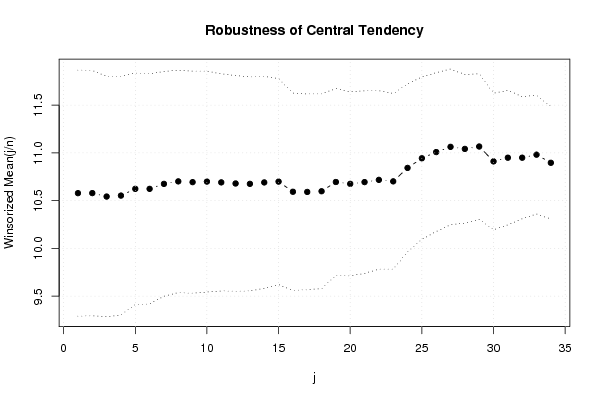
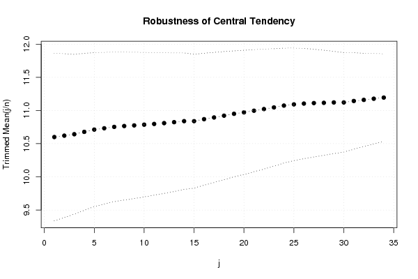
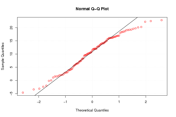
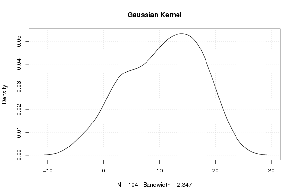
| Charts produced by software: | |||||||||||||||||||||||||||||||||||||||||||||||||||||||||||||||||||||||||||||||||||||||||||||||||||||||||||||||||||||||||||||||||||||||||||||||||||||||||||||||||||||||||||||||||||||||||||||||||||||||||||||||||||||||||||||||||||||||||||||||||||||||||||||||||||||||||||||||||||||||||||||||||||||||||||||||||||||||||||||||||||||||||||||||||||||||||||||||||||||||||||||||||||||||||||||||||||||||||||||||||||||||||||||||||||||||||||||||||||||||||||||||||||||||||||||||||||||||||||||||||||||||||||||||||||||||||||||||||||||||||||||||||||||||||||||||||||||||||||||||||||||||||||||||||||||||||||||||||||||||||||||||||||||||||||||||||||||||||||||||||||||||||||||||||||||||||||||||||||||||||||||||||||||||||||||||||||||||||||||||||||||||||||||||||||||||||||||||||||||||||||||||||||||||||||||||||||||||||||||||||||||||||||||||||||||||||||||||||||||||||||||||||||||||||||||||||||||||||||||||||||||||||||||||||||||||||||||||||||||||||||||||||||||||||||||||||||||||||||||||||||||||||||||||||||||||||||||||||||||||
| |||||||||||||||||||||||||||||||||||||||||||||||||||||||||||||||||||||||||||||||||||||||||||||||||||||||||||||||||||||||||||||||||||||||||||||||||||||||||||||||||||||||||||||||||||||||||||||||||||||||||||||||||||||||||||||||||||||||||||||||||||||||||||||||||||||||||||||||||||||||||||||||||||||||||||||||||||||||||||||||||||||||||||||||||||||||||||||||||||||||||||||||||||||||||||||||||||||||||||||||||||||||||||||||||||||||||||||||||||||||||||||||||||||||||||||||||||||||||||||||||||||||||||||||||||||||||||||||||||||||||||||||||||||||||||||||||||||||||||||||||||||||||||||||||||||||||||||||||||||||||||||||||||||||||||||||||||||||||||||||||||||||||||||||||||||||||||||||||||||||||||||||||||||||||||||||||||||||||||||||||||||||||||||||||||||||||||||||||||||||||||||||||||||||||||||||||||||||||||||||||||||||||||||||||||||||||||||||||||||||||||||||||||||||||||||||||||||||||||||||||||||||||||||||||||||||||||||||||||||||||||||||||||||||||||||||||||||||||||||||||||||||||||||||||||||||||||||||||||||||
| Parameters (Session): | |||||||||||||||||||||||||||||||||||||||||||||||||||||||||||||||||||||||||||||||||||||||||||||||||||||||||||||||||||||||||||||||||||||||||||||||||||||||||||||||||||||||||||||||||||||||||||||||||||||||||||||||||||||||||||||||||||||||||||||||||||||||||||||||||||||||||||||||||||||||||||||||||||||||||||||||||||||||||||||||||||||||||||||||||||||||||||||||||||||||||||||||||||||||||||||||||||||||||||||||||||||||||||||||||||||||||||||||||||||||||||||||||||||||||||||||||||||||||||||||||||||||||||||||||||||||||||||||||||||||||||||||||||||||||||||||||||||||||||||||||||||||||||||||||||||||||||||||||||||||||||||||||||||||||||||||||||||||||||||||||||||||||||||||||||||||||||||||||||||||||||||||||||||||||||||||||||||||||||||||||||||||||||||||||||||||||||||||||||||||||||||||||||||||||||||||||||||||||||||||||||||||||||||||||||||||||||||||||||||||||||||||||||||||||||||||||||||||||||||||||||||||||||||||||||||||||||||||||||||||||||||||||||||||||||||||||||||||||||||||||||||||||||||||||||||||||||||||||||||||
| Parameters (R input): | |||||||||||||||||||||||||||||||||||||||||||||||||||||||||||||||||||||||||||||||||||||||||||||||||||||||||||||||||||||||||||||||||||||||||||||||||||||||||||||||||||||||||||||||||||||||||||||||||||||||||||||||||||||||||||||||||||||||||||||||||||||||||||||||||||||||||||||||||||||||||||||||||||||||||||||||||||||||||||||||||||||||||||||||||||||||||||||||||||||||||||||||||||||||||||||||||||||||||||||||||||||||||||||||||||||||||||||||||||||||||||||||||||||||||||||||||||||||||||||||||||||||||||||||||||||||||||||||||||||||||||||||||||||||||||||||||||||||||||||||||||||||||||||||||||||||||||||||||||||||||||||||||||||||||||||||||||||||||||||||||||||||||||||||||||||||||||||||||||||||||||||||||||||||||||||||||||||||||||||||||||||||||||||||||||||||||||||||||||||||||||||||||||||||||||||||||||||||||||||||||||||||||||||||||||||||||||||||||||||||||||||||||||||||||||||||||||||||||||||||||||||||||||||||||||||||||||||||||||||||||||||||||||||||||||||||||||||||||||||||||||||||||||||||||||||||||||||||||||||||
| R code (references can be found in the software module): | |||||||||||||||||||||||||||||||||||||||||||||||||||||||||||||||||||||||||||||||||||||||||||||||||||||||||||||||||||||||||||||||||||||||||||||||||||||||||||||||||||||||||||||||||||||||||||||||||||||||||||||||||||||||||||||||||||||||||||||||||||||||||||||||||||||||||||||||||||||||||||||||||||||||||||||||||||||||||||||||||||||||||||||||||||||||||||||||||||||||||||||||||||||||||||||||||||||||||||||||||||||||||||||||||||||||||||||||||||||||||||||||||||||||||||||||||||||||||||||||||||||||||||||||||||||||||||||||||||||||||||||||||||||||||||||||||||||||||||||||||||||||||||||||||||||||||||||||||||||||||||||||||||||||||||||||||||||||||||||||||||||||||||||||||||||||||||||||||||||||||||||||||||||||||||||||||||||||||||||||||||||||||||||||||||||||||||||||||||||||||||||||||||||||||||||||||||||||||||||||||||||||||||||||||||||||||||||||||||||||||||||||||||||||||||||||||||||||||||||||||||||||||||||||||||||||||||||||||||||||||||||||||||||||||||||||||||||||||||||||||||||||||||||||||||||||||||||||||||||||
| load(file='createtable')
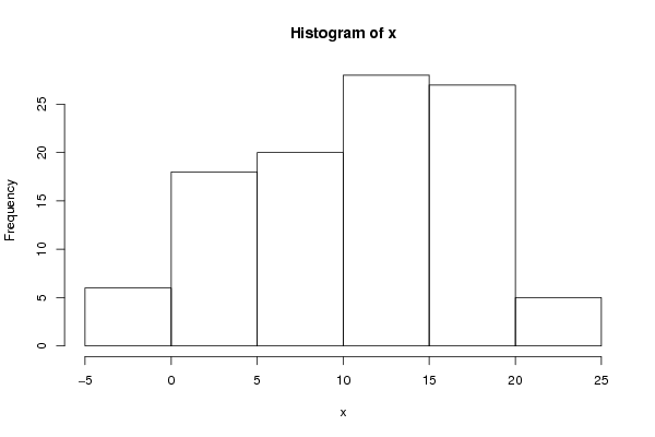
x <-sort(x[!is.na(x)]) num <- 50 res <- array(NA,dim=c(num,3)) geomean <- function(x) { return(exp(mean(log(x)))) } harmean <- function(x) { return(1/mean(1/x)) } quamean <- function(x) { return(sqrt(mean(x*x))) } winmean <- function(x) { x <-sort(x[!is.na(x)]) n<-length(x) denom <- 3 nodenom <- n/denom if (nodenom>40) denom <- n/40 sqrtn = sqrt(n) roundnodenom = floor(nodenom) win <- array(NA,dim=c(roundnodenom,2)) for (j in 1:roundnodenom) { win[j,1] <- (j*x[j+1]+sum(x[(j+1):(n-j)])+j*x[n-j])/n win[j,2] <- sd(c(rep(x[j+1],j),x[(j+1):(n-j)],rep(x[n-j],j)))/sqrtn } return(win) } trimean <- function(x) { x <-sort(x[!is.na(x)]) n<-length(x) denom <- 3 nodenom <- n/denom if (nodenom>40) denom <- n/40 sqrtn = sqrt(n) roundnodenom = floor(nodenom) tri <- array(NA,dim=c(roundnodenom,2)) for (j in 1:roundnodenom) { tri[j,1] <- mean(x,trim=j/n) tri[j,2] <- sd(x[(j+1):(n-j)]) / sqrt(n-j*2) } return(tri) } midrange <- function(x) { return((max(x)+min(x))/2) } q1 <- function(data,n,p,i,f) { np <- n*p; i <<- floor(np) f <<- np - i qvalue <- (1-f)*data[i] + f*data[i+1] } q2 <- function(data,n,p,i,f) { np <- (n+1)*p i <<- floor(np) f <<- np - i qvalue <- (1-f)*data[i] + f*data[i+1] } q3 <- function(data,n,p,i,f) { np <- n*p i <<- floor(np) f <<- np - i if (f==0) { qvalue <- data[i] } else { qvalue <- data[i+1] } } q4 <- function(data,n,p,i,f) { np <- n*p i <<- floor(np) f <<- np - i if (f==0) { qvalue <- (data[i]+data[i+1])/2 } else { qvalue <- data[i+1] } } q5 <- function(data,n,p,i,f) { np <- (n-1)*p i <<- floor(np) f <<- np - i if (f==0) { qvalue <- data[i+1] } else { qvalue <- data[i+1] + f*(data[i+2]-data[i+1]) } } q6 <- function(data,n,p,i,f) { np <- n*p+0.5 i <<- floor(np) f <<- np - i qvalue <- data[i] } q7 <- function(data,n,p,i,f) { np <- (n+1)*p i <<- floor(np) f <<- np - i if (f==0) { qvalue <- data[i] } else { qvalue <- f*data[i] + (1-f)*data[i+1] } } q8 <- function(data,n,p,i,f) { np <- (n+1)*p i <<- floor(np) f <<- np - i if (f==0) { qvalue <- data[i] } else { if (f == 0.5) { qvalue <- (data[i]+data[i+1])/2 } else { if (f < 0.5) { qvalue <- data[i] } else { qvalue <- data[i+1] } } } } iqd <- function(x,def) { x <-sort(x[!is.na(x)]) n<-length(x) if (def==1) { qvalue1 <- q1(x,n,0.25,i,f) qvalue3 <- q1(x,n,0.75,i,f) } if (def==2) { qvalue1 <- q2(x,n,0.25,i,f) qvalue3 <- q2(x,n,0.75,i,f) } if (def==3) { qvalue1 <- q3(x,n,0.25,i,f) qvalue3 <- q3(x,n,0.75,i,f) } if (def==4) { qvalue1 <- q4(x,n,0.25,i,f) qvalue3 <- q4(x,n,0.75,i,f) } if (def==5) { qvalue1 <- q5(x,n,0.25,i,f) qvalue3 <- q5(x,n,0.75,i,f) } if (def==6) { qvalue1 <- q6(x,n,0.25,i,f) qvalue3 <- q6(x,n,0.75,i,f) } if (def==7) { qvalue1 <- q7(x,n,0.25,i,f) qvalue3 <- q7(x,n,0.75,i,f) } if (def==8) { qvalue1 <- q8(x,n,0.25,i,f) qvalue3 <- q8(x,n,0.75,i,f) } iqdiff <- qvalue3 - qvalue1 return(c(iqdiff,iqdiff/2,iqdiff/(qvalue3 + qvalue1))) } midmean <- function(x,def) { x <-sort(x[!is.na(x)]) n<-length(x) if (def==1) { qvalue1 <- q1(x,n,0.25,i,f) qvalue3 <- q1(x,n,0.75,i,f) } if (def==2) { qvalue1 <- q2(x,n,0.25,i,f) qvalue3 <- q2(x,n,0.75,i,f) } if (def==3) { qvalue1 <- q3(x,n,0.25,i,f) qvalue3 <- q3(x,n,0.75,i,f) } if (def==4) { qvalue1 <- q4(x,n,0.25,i,f) qvalue3 <- q4(x,n,0.75,i,f) } if (def==5) { qvalue1 <- q5(x,n,0.25,i,f) qvalue3 <- q5(x,n,0.75,i,f) } if (def==6) { qvalue1 <- q6(x,n,0.25,i,f) qvalue3 <- q6(x,n,0.75,i,f) } if (def==7) { qvalue1 <- q7(x,n,0.25,i,f) qvalue3 <- q7(x,n,0.75,i,f) } if (def==8) { qvalue1 <- q8(x,n,0.25,i,f) qvalue3 <- q8(x,n,0.75,i,f) } midm <- 0 myn <- 0 roundno4 <- round(n/4) round3no4 <- round(3*n/4) for (i in 1:n) { if ((x[i]>=qvalue1) & (x[i]<=qvalue3)){ midm = midm + x[i] myn = myn + 1 } } midm = midm / myn return(midm) } range <- max(x) - min(x) lx <- length(x) biasf <- (lx-1)/lx varx <- var(x) bvarx <- varx*biasf sdx <- sqrt(varx) mx <- mean(x) bsdx <- sqrt(bvarx) x2 <- x*x mse0 <- sum(x2)/lx xmm <- x-mx xmm2 <- xmm*xmm msem <- sum(xmm2)/lx axmm <- abs(x - mx) medx <- median(x) axmmed <- abs(x - medx) xmmed <- x - medx xmmed2 <- xmmed*xmmed msemed <- sum(xmmed2)/lx qarr <- array(NA,dim=c(8,3)) for (j in 1:8) { qarr[j,] <- iqd(x,j) } sdpo <- 0 adpo <- 0 for (i in 1:(lx-1)) { for (j in (i+1):lx) { ldi <- x[i]-x[j] aldi <- abs(ldi) sdpo = sdpo + ldi * ldi adpo = adpo + aldi } } denom <- (lx*(lx-1)/2) sdpo = sdpo / denom adpo = adpo / denom gmd <- 0 for (i in 1:lx) { for (j in 1:lx) { ldi <- abs(x[i]-x[j]) gmd = gmd + ldi } } gmd <- gmd / (lx*(lx-1)) sumx <- sum(x) pk <- x / sumx ck <- cumsum(pk) dk <- array(NA,dim=lx) for (i in 1:lx) { if (ck[i] <= 0.5) dk[i] <- ck[i] else dk[i] <- 1 - ck[i] } bigd <- sum(dk) * 2 / (lx-1) iod <- 1 - sum(pk*pk) res[1,] <- c('Absolute range','http://www.xycoon.com/absolute.htm', range) res[2,] <- c('Relative range (unbiased)','http://www.xycoon.com/relative.htm', range/sd(x)) res[3,] <- c('Relative range (biased)','http://www.xycoon.com/relative.htm', range/sqrt(varx*biasf)) res[4,] <- c('Variance (unbiased)','http://www.xycoon.com/unbiased.htm', varx) res[5,] <- c('Variance (biased)','http://www.xycoon.com/biased.htm', bvarx) res[6,] <- c('Standard Deviation (unbiased)','http://www.xycoon.com/unbiased1.htm', sdx) res[7,] <- c('Standard Deviation (biased)','http://www.xycoon.com/biased1.htm', bsdx) res[8,] <- c('Coefficient of Variation (unbiased)','http://www.xycoon.com/variation.htm', sdx/mx) res[9,] <- c('Coefficient of Variation (biased)','http://www.xycoon.com/variation.htm', bsdx/mx) res[10,] <- c('Mean Squared Error (MSE versus 0)','http://www.xycoon.com/mse.htm', mse0) res[11,] <- c('Mean Squared Error (MSE versus Mean)','http://www.xycoon.com/mse.htm', msem) res[12,] <- c('Mean Absolute Deviation from Mean (MAD Mean)', 'http://www.xycoon.com/mean2.htm', sum(axmm)/lx) res[13,] <- c('Mean Absolute Deviation from Median (MAD Median)', 'http://www.xycoon.com/median1.htm', sum(axmmed)/lx) res[14,] <- c('Median Absolute Deviation from Mean', 'http://www.xycoon.com/mean3.htm', median(axmm)) res[15,] <- c('Median Absolute Deviation from Median', 'http://www.xycoon.com/median2.htm', median(axmmed)) res[16,] <- c('Mean Squared Deviation from Mean', 'http://www.xycoon.com/mean1.htm', msem) res[17,] <- c('Mean Squared Deviation from Median', 'http://www.xycoon.com/median.htm', msemed) mylink1 <- hyperlink('http://www.xycoon.com/difference.htm','Interquartile Difference','') mylink2 <- paste(mylink1,hyperlink('http://www.xycoon.com/method_1.htm','(Weighted Average at Xnp)',''),sep=' ') res[18,] <- c('', mylink2, qarr[1,1]) mylink2 <- paste(mylink1,hyperlink('http://www.xycoon.com/method_2.htm','(Weighted Average at X(n+1)p)',''),sep=' ') res[19,] <- c('', mylink2, qarr[2,1]) mylink2 <- paste(mylink1,hyperlink('http://www.xycoon.com/method_3.htm','(Empirical Distribution Function)',''),sep=' ') res[20,] <- c('', mylink2, qarr[3,1]) mylink2 <- paste(mylink1,hyperlink('http://www.xycoon.com/method_4.htm','(Empirical Distribution Function - Averaging)',''),sep=' ') res[21,] <- c('', mylink2, qarr[4,1]) mylink2 <- paste(mylink1,hyperlink('http://www.xycoon.com/method_5.htm','(Empirical Distribution Function - Interpolation)',''),sep=' ') res[22,] <- c('', mylink2, qarr[5,1]) mylink2 <- paste(mylink1,hyperlink('http://www.xycoon.com/method_6.htm','(Closest Observation)',''),sep=' ') res[23,] <- c('', mylink2, qarr[6,1]) mylink2 <- paste(mylink1,hyperlink('http://www.xycoon.com/method_7.htm','(True Basic - Statistics Graphics Toolkit)',''),sep=' ') res[24,] <- c('', mylink2, qarr[7,1]) mylink2 <- paste(mylink1,hyperlink('http://www.xycoon.com/method_8.htm','(MS Excel (old versions))',''),sep=' ') res[25,] <- c('', mylink2, qarr[8,1]) mylink1 <- hyperlink('http://www.xycoon.com/deviation.htm','Semi Interquartile Difference','') mylink2 <- paste(mylink1,hyperlink('http://www.xycoon.com/method_1.htm','(Weighted Average at Xnp)',''),sep=' ') res[26,] <- c('', mylink2, qarr[1,2]) mylink2 <- paste(mylink1,hyperlink('http://www.xycoon.com/method_2.htm','(Weighted Average at X(n+1)p)',''),sep=' ') res[27,] <- c('', mylink2, qarr[2,2]) mylink2 <- paste(mylink1,hyperlink('http://www.xycoon.com/method_3.htm','(Empirical Distribution Function)',''),sep=' ') res[28,] <- c('', mylink2, qarr[3,2]) mylink2 <- paste(mylink1,hyperlink('http://www.xycoon.com/method_4.htm','(Empirical Distribution Function - Averaging)',''),sep=' ') res[29,] <- c('', mylink2, qarr[4,2]) mylink2 <- paste(mylink1,hyperlink('http://www.xycoon.com/method_5.htm','(Empirical Distribution Function - Interpolation)',''),sep=' ') res[30,] <- c('', mylink2, qarr[5,2]) mylink2 <- paste(mylink1,hyperlink('http://www.xycoon.com/method_6.htm','(Closest Observation)',''),sep=' ') res[31,] <- c('', mylink2, qarr[6,2]) mylink2 <- paste(mylink1,hyperlink('http://www.xycoon.com/method_7.htm','(True Basic - Statistics Graphics Toolkit)',''),sep=' ') res[32,] <- c('', mylink2, qarr[7,2]) mylink2 <- paste(mylink1,hyperlink('http://www.xycoon.com/method_8.htm','(MS Excel (old versions))',''),sep=' ') res[33,] <- c('', mylink2, qarr[8,2]) mylink1 <- hyperlink('http://www.xycoon.com/variation1.htm','Coefficient of Quartile Variation','') mylink2 <- paste(mylink1,hyperlink('http://www.xycoon.com/method_1.htm','(Weighted Average at Xnp)',''),sep=' ') res[34,] <- c('', mylink2, qarr[1,3]) mylink2 <- paste(mylink1,hyperlink('http://www.xycoon.com/method_2.htm','(Weighted Average at X(n+1)p)',''),sep=' ') res[35,] <- c('', mylink2, qarr[2,3]) mylink2 <- paste(mylink1,hyperlink('http://www.xycoon.com/method_3.htm','(Empirical Distribution Function)',''),sep=' ') res[36,] <- c('', mylink2, qarr[3,3]) mylink2 <- paste(mylink1,hyperlink('http://www.xycoon.com/method_4.htm','(Empirical Distribution Function - Averaging)',''),sep=' ') res[37,] <- c('', mylink2, qarr[4,3]) mylink2 <- paste(mylink1,hyperlink('http://www.xycoon.com/method_5.htm','(Empirical Distribution Function - Interpolation)',''),sep=' ') res[38,] <- c('', mylink2, qarr[5,3]) mylink2 <- paste(mylink1,hyperlink('http://www.xycoon.com/method_6.htm','(Closest Observation)',''),sep=' ') res[39,] <- c('', mylink2, qarr[6,3]) mylink2 <- paste(mylink1,hyperlink('http://www.xycoon.com/method_7.htm','(True Basic - Statistics Graphics Toolkit)',''),sep=' ') res[40,] <- c('', mylink2, qarr[7,3]) mylink2 <- paste(mylink1,hyperlink('http://www.xycoon.com/method_8.htm','(MS Excel (old versions))',''),sep=' ') res[41,] <- c('', mylink2, qarr[8,3]) res[42,] <- c('Number of all Pairs of Observations', 'http://www.xycoon.com/pair_numbers.htm', lx*(lx-1)/2) res[43,] <- c('Squared Differences between all Pairs of Observations', 'http://www.xycoon.com/squared_differences.htm', sdpo) res[44,] <- c('Mean Absolute Differences between all Pairs of Observations', 'http://www.xycoon.com/mean_abs_differences.htm', adpo) res[45,] <- c('Gini Mean Difference', 'http://www.xycoon.com/gini_mean_difference.htm', gmd) res[46,] <- c('Leik Measure of Dispersion', 'http://www.xycoon.com/leiks_d.htm', bigd) res[47,] <- c('Index of Diversity', 'http://www.xycoon.com/diversity.htm', iod) res[48,] <- c('Index of Qualitative Variation', 'http://www.xycoon.com/qualitative_variation.htm', iod*lx/(lx-1)) res[49,] <- c('Coefficient of Dispersion', 'http://www.xycoon.com/dispersion.htm', sum(axmm)/lx/medx) res[50,] <- c('Observations', '', lx) res (arm <- mean(x)) sqrtn <- sqrt(length(x)) (armse <- sd(x) / sqrtn) (armose <- arm / armse) (geo <- geomean(x)) (har <- harmean(x)) (qua <- quamean(x)) (win <- winmean(x)) (tri <- trimean(x)) (midr <- midrange(x)) midm <- array(NA,dim=8) for (j in 1:8) midm[j] <- midmean(x,j) midm bitmap(file='test1.png') lb <- win[,1] - 2*win[,2] ub <- win[,1] + 2*win[,2] if ((ylimmin == '') | (ylimmax == '')) plot(win[,1],type='b',main='Robustness of Central Tendency', xlab='j', pch=19, ylab='Winsorized Mean(j/n)', ylim=c(min(lb),max(ub))) else plot(win[,1],type='l',main='Robustness of Central Tendency', xlab='j', pch=19, ylab='Winsorized Mean(j/n)', ylim=c(ylimmin,ylimmax)) lines(ub,lty=3) lines(lb,lty=3) grid() dev.off() bitmap(file='test2.png') lb <- tri[,1] - 2*tri[,2] ub <- tri[,1] + 2*tri[,2] if ((ylimmin == '') | (ylimmax == '')) plot(tri[,1],type='b',main='Robustness of Central Tendency', xlab='j', pch=19, ylab='Trimmed Mean(j/n)', ylim=c(min(lb),max(ub))) else plot(tri[,1],type='l',main='Robustness of Central Tendency', xlab='j', pch=19, ylab='Trimmed Mean(j/n)', ylim=c(ylimmin,ylimmax)) lines(ub,lty=3) lines(lb,lty=3) grid() dev.off() a<-table.start() a<-table.row.start(a) a<-table.element(a,'Central Tendency - Ungrouped Data',4,TRUE) a<-table.row.end(a) a<-table.row.start(a) a<-table.element(a,'Measure',header=TRUE) a<-table.element(a,'Value',header=TRUE) a<-table.element(a,'S.E.',header=TRUE) a<-table.element(a,'Value/S.E.',header=TRUE) a<-table.row.end(a) a<-table.row.start(a) a<-table.element(a,hyperlink('http://www.xycoon.com/arithmetic_mean.htm', 'Arithmetic Mean', 'click to view the definition of the Arithmetic Mean'),header=TRUE) a<-table.element(a,arm) a<-table.element(a,hyperlink('http://www.xycoon.com/arithmetic_mean_standard_error.htm', armse, 'click to view the definition of the Standard Error of the Arithmetic Mean')) a<-table.element(a,armose) a<-table.row.end(a) a<-table.row.start(a) a<-table.element(a,hyperlink('http://www.xycoon.com/geometric_mean.htm', 'Geometric Mean', 'click to view the definition of the Geometric Mean'),header=TRUE) a<-table.element(a,geo) a<-table.element(a,'') a<-table.element(a,'') a<-table.row.end(a) a<-table.row.start(a) a<-table.element(a,hyperlink('http://www.xycoon.com/harmonic_mean.htm', 'Harmonic Mean', 'click to view the definition of the Harmonic Mean'),header=TRUE) a<-table.element(a,har) a<-table.element(a,'') a<-table.element(a,'') a<-table.row.end(a) a<-table.row.start(a) a<-table.element(a,hyperlink('http://www.xycoon.com/quadratic_mean.htm', 'Quadratic Mean', 'click to view the definition of the Quadratic Mean'),header=TRUE) a<-table.element(a,qua) a<-table.element(a,'') a<-table.element(a,'') a<-table.row.end(a) for (j in 1:length(win[,1])) { a<-table.row.start(a) mylabel <- paste('Winsorized Mean (',j) mylabel <- paste(mylabel,'/') mylabel <- paste(mylabel,length(win[,1])) mylabel <- paste(mylabel,')') a<-table.element(a,hyperlink('http://www.xycoon.com/winsorized_mean.htm', mylabel, 'click to view the definition of the Winsorized Mean'),header=TRUE) a<-table.element(a,win[j,1]) a<-table.element(a,win[j,2]) a<-table.element(a,win[j,1]/win[j,2]) a<-table.row.end(a) } for (j in 1:length(tri[,1])) { a<-table.row.start(a) mylabel <- paste('Trimmed Mean (',j) mylabel <- paste(mylabel,'/') mylabel <- paste(mylabel,length(tri[,1])) mylabel <- paste(mylabel,')') a<-table.element(a,hyperlink('http://www.xycoon.com/arithmetic_mean.htm', mylabel, 'click to view the definition of the Trimmed Mean'),header=TRUE) a<-table.element(a,tri[j,1]) a<-table.element(a,tri[j,2]) a<-table.element(a,tri[j,1]/tri[j,2]) a<-table.row.end(a) } a<-table.row.start(a) a<-table.element(a,hyperlink('http://www.xycoon.com/median_1.htm', 'Median', 'click to view the definition of the Median'),header=TRUE) a<-table.element(a,median(x)) a<-table.element(a,'') a<-table.element(a,'') a<-table.row.end(a) a<-table.row.start(a) a<-table.element(a,hyperlink('http://www.xycoon.com/midrange.htm', 'Midrange', 'click to view the definition of the Midrange'),header=TRUE) a<-table.element(a,midr) a<-table.element(a,'') a<-table.element(a,'') a<-table.row.end(a) a<-table.row.start(a) mymid <- hyperlink('http://www.xycoon.com/midmean.htm', 'Midmean', 'click to view the definition of the Midmean') mylabel <- paste(mymid,hyperlink('http://www.xycoon.com/method_1.htm','Weighted Average at Xnp',''),sep=' - ') a<-table.element(a,mylabel,header=TRUE) a<-table.element(a,midm[1]) a<-table.element(a,'') a<-table.element(a,'') a<-table.row.end(a) a<-table.row.start(a) mymid <- hyperlink('http://www.xycoon.com/midmean.htm', 'Midmean', 'click to view the definition of the Midmean') mylabel <- paste(mymid,hyperlink('http://www.xycoon.com/method_2.htm','Weighted Average at X(n+1)p',''),sep=' - ') a<-table.element(a,mylabel,header=TRUE) a<-table.element(a,midm[2]) a<-table.element(a,'') a<-table.element(a,'') a<-table.row.end(a) a<-table.row.start(a) mymid <- hyperlink('http://www.xycoon.com/midmean.htm', 'Midmean', 'click to view the definition of the Midmean') mylabel <- paste(mymid,hyperlink('http://www.xycoon.com/method_3.htm','Empirical Distribution Function',''),sep=' - ') a<-table.element(a,mylabel,header=TRUE) a<-table.element(a,midm[3]) a<-table.element(a,'') a<-table.element(a,'') a<-table.row.end(a) a<-table.row.start(a) mymid <- hyperlink('http://www.xycoon.com/midmean.htm', 'Midmean', 'click to view the definition of the Midmean') mylabel <- paste(mymid,hyperlink('http://www.xycoon.com/method_4.htm','Empirical Distribution Function - Averaging',''),sep=' - ') a<-table.element(a,mylabel,header=TRUE) a<-table.element(a,midm[4]) a<-table.element(a,'') a<-table.element(a,'') a<-table.row.end(a) a<-table.row.start(a) mymid <- hyperlink('http://www.xycoon.com/midmean.htm', 'Midmean', 'click to view the definition of the Midmean') mylabel <- paste(mymid,hyperlink('http://www.xycoon.com/method_5.htm','Empirical Distribution Function - Interpolation',''),sep=' - ') a<-table.element(a,mylabel,header=TRUE) a<-table.element(a,midm[5]) a<-table.element(a,'') a<-table.element(a,'') a<-table.row.end(a) a<-table.row.start(a) mymid <- hyperlink('http://www.xycoon.com/midmean.htm', 'Midmean', 'click to view the definition of the Midmean') mylabel <- paste(mymid,hyperlink('http://www.xycoon.com/method_6.htm','Closest Observation',''),sep=' - ') a<-table.element(a,mylabel,header=TRUE) a<-table.element(a,midm[6]) a<-table.element(a,'') a<-table.element(a,'') a<-table.row.end(a) a<-table.row.start(a) mymid <- hyperlink('http://www.xycoon.com/midmean.htm', 'Midmean', 'click to view the definition of the Midmean') mylabel <- paste(mymid,hyperlink('http://www.xycoon.com/method_7.htm','True Basic - Statistics Graphics Toolkit',''),sep=' - ') a<-table.element(a,mylabel,header=TRUE) a<-table.element(a,midm[7]) a<-table.element(a,'') a<-table.element(a,'') a<-table.row.end(a) a<-table.row.start(a) mymid <- hyperlink('http://www.xycoon.com/midmean.htm', 'Midmean', 'click to view the definition of the Midmean') mylabel <- paste(mymid,hyperlink('http://www.xycoon.com/method_8.htm','MS Excel (old versions)',''),sep=' - ') a<-table.element(a,mylabel,header=TRUE) a<-table.element(a,midm[8]) a<-table.element(a,'') a<-table.element(a,'') a<-table.row.end(a) a<-table.row.start(a) a<-table.element(a,'Number of observations',header=TRUE) a<-table.element(a,length(x)) a<-table.element(a,'') a<-table.element(a,'') a<-table.row.end(a) a<-table.end(a) table.save(a,file='mytable.tab') a<-table.start() a<-table.row.start(a) a<-table.element(a,'Variability - Ungrouped Data',2,TRUE) a<-table.row.end(a) for (i in 1:num) { a<-table.row.start(a) if (res[i,1] != '') { a<-table.element(a,hyperlink(res[i,2],res[i,1],''),header=TRUE) } else { a<-table.element(a,res[i,2],header=TRUE) } a<-table.element(a,res[i,3]) a<-table.row.end(a) } a<-table.end(a) table.save(a,file='mytable1.tab') lx <- length(x) qval <- array(NA,dim=c(99,8)) mystep <- 25 mystart <- 25 if (lx>10){ mystep=10 mystart=10 } if (lx>20){ mystep=5 mystart=5 } if (lx>50){ mystep=2 mystart=2 } if (lx>=100){ mystep=1 mystart=1 } for (perc in seq(mystart,99,mystep)) { qval[perc,1] <- q1(x,lx,perc/100,i,f) qval[perc,2] <- q2(x,lx,perc/100,i,f) qval[perc,3] <- q3(x,lx,perc/100,i,f) qval[perc,4] <- q4(x,lx,perc/100,i,f) qval[perc,5] <- q5(x,lx,perc/100,i,f) qval[perc,6] <- q6(x,lx,perc/100,i,f) qval[perc,7] <- q7(x,lx,perc/100,i,f) qval[perc,8] <- q8(x,lx,perc/100,i,f) } bitmap(file='test3.png') myqqnorm <- qqnorm(x,col=2) qqline(x) grid() dev.off() a<-table.start() a<-table.row.start(a) a<-table.element(a,'Percentiles - Ungrouped Data',9,TRUE) a<-table.row.end(a) a<-table.row.start(a) a<-table.element(a,'p',1,TRUE) a<-table.element(a,hyperlink('http://www.xycoon.com/method_1.htm', 'Weighted Average at Xnp',''),1,TRUE) a<-table.element(a,hyperlink('http://www.xycoon.com/method_2.htm','Weighted Average at X(n+1)p',''),1,TRUE) a<-table.element(a,hyperlink('http://www.xycoon.com/method_3.htm','Empirical Distribution Function',''),1,TRUE) a<-table.element(a,hyperlink('http://www.xycoon.com/method_4.htm','Empirical Distribution Function - Averaging',''),1,TRUE) a<-table.element(a,hyperlink('http://www.xycoon.com/method_5.htm','Empirical Distribution Function - Interpolation',''),1,TRUE) a<-table.element(a,hyperlink('http://www.xycoon.com/method_6.htm','Closest Observation',''),1,TRUE) a<-table.element(a,hyperlink('http://www.xycoon.com/method_7.htm','True Basic - Statistics Graphics Toolkit',''),1,TRUE) a<-table.element(a,hyperlink('http://www.xycoon.com/method_8.htm','MS Excel (old versions)',''),1,TRUE) a<-table.row.end(a) for (perc in seq(mystart,99,mystep)) { a<-table.row.start(a) a<-table.element(a,round(perc/100,2),1,TRUE) for (j in 1:8) { a<-table.element(a,round(qval[perc,j],6)) } a<-table.row.end(a) } a<-table.end(a) table.save(a,file='mytable2.tab') bitmap(file='histogram1.png') myhist<-hist(x) dev.off() myhist n <- length(x) a<-table.start() a<-table.row.start(a) a<-table.element(a,hyperlink('http://www.xycoon.com/histogram.htm','Frequency Table (Histogram)',''),6,TRUE) a<-table.row.end(a) a<-table.row.start(a) a<-table.element(a,'Bins',header=TRUE) a<-table.element(a,'Midpoint',header=TRUE) a<-table.element(a,'Abs. Frequency',header=TRUE) a<-table.element(a,'Rel. Frequency',header=TRUE) a<-table.element(a,'Cumul. Rel. Freq.',header=TRUE) a<-table.element(a,'Density',header=TRUE) a<-table.row.end(a) crf <- 0 mybracket <- '[' mynumrows <- (length(myhist$breaks)-1) for (i in 1:mynumrows) { a<-table.row.start(a) if (i == 1) dum <- paste('[',myhist$breaks[i],sep='') else dum <- paste(mybracket,myhist$breaks[i],sep='') dum <- paste(dum,myhist$breaks[i+1],sep=',') if (i==mynumrows) dum <- paste(dum,']',sep='') else dum <- paste(dum,mybracket,sep='') a<-table.element(a,dum,header=TRUE) a<-table.element(a,myhist$mids[i]) a<-table.element(a,myhist$counts[i]) rf <- myhist$counts[i]/n crf <- crf + rf a<-table.element(a,round(rf,6)) a<-table.element(a,round(crf,6)) a<-table.element(a,round(myhist$density[i],6)) a<-table.row.end(a) } a<-table.end(a) table.save(a,file='mytable5.tab') bitmap(file='density1.png') mydensity1<-density(x,kernel='gaussian',na.rm=TRUE) plot(mydensity1,main='Gaussian Kernel') grid() dev.off() mydensity1 a<-table.start() a<-table.row.start(a) a<-table.element(a,'Properties of Density Trace',2,TRUE) a<-table.row.end(a) a<-table.row.start(a) a<-table.element(a,'Bandwidth',header=TRUE) a<-table.element(a,mydensity1$bw) a<-table.row.end(a) a<-table.row.start(a) a<-table.element(a,'#Observations',header=TRUE) a<-table.element(a,mydensity1$n) a<-table.row.end(a) a<-table.end(a) table.save(a,file='mytable4.tab') | |||||||||||||||||||||||||||||||||||||||||||||||||||||||||||||||||||||||||||||||||||||||||||||||||||||||||||||||||||||||||||||||||||||||||||||||||||||||||||||||||||||||||||||||||||||||||||||||||||||||||||||||||||||||||||||||||||||||||||||||||||||||||||||||||||||||||||||||||||||||||||||||||||||||||||||||||||||||||||||||||||||||||||||||||||||||||||||||||||||||||||||||||||||||||||||||||||||||||||||||||||||||||||||||||||||||||||||||||||||||||||||||||||||||||||||||||||||||||||||||||||||||||||||||||||||||||||||||||||||||||||||||||||||||||||||||||||||||||||||||||||||||||||||||||||||||||||||||||||||||||||||||||||||||||||||||||||||||||||||||||||||||||||||||||||||||||||||||||||||||||||||||||||||||||||||||||||||||||||||||||||||||||||||||||||||||||||||||||||||||||||||||||||||||||||||||||||||||||||||||||||||||||||||||||||||||||||||||||||||||||||||||||||||||||||||||||||||||||||||||||||||||||||||||||||||||||||||||||||||||||||||||||||||||||||||||||||||||||||||||||||||||||||||||||||||||||||||||||||||||
Copyright

This work is licensed under a
Creative Commons Attribution-Noncommercial-Share Alike 3.0 License.
Software written by Ed van Stee & Patrick Wessa
Disclaimer
Information provided on this web site is provided "AS IS" without warranty of any kind, either express or implied, including, without limitation, warranties of merchantability, fitness for a particular purpose, and noninfringement. We use reasonable efforts to include accurate and timely information and periodically update the information, and software without notice. However, we make no warranties or representations as to the accuracy or completeness of such information (or software), and we assume no liability or responsibility for errors or omissions in the content of this web site, or any software bugs in online applications. Your use of this web site is AT YOUR OWN RISK. Under no circumstances and under no legal theory shall we be liable to you or any other person for any direct, indirect, special, incidental, exemplary, or consequential damages arising from your access to, or use of, this web site.
Privacy Policy
We may request personal information to be submitted to our servers in order to be able to:
- personalize online software applications according to your needs
- enforce strict security rules with respect to the data that you upload (e.g. statistical data)
- manage user sessions of online applications
- alert you about important changes or upgrades in resources or applications
We NEVER allow other companies to directly offer registered users information about their products and services. Banner references and hyperlinks of third parties NEVER contain any personal data of the visitor.
We do NOT sell, nor transmit by any means, personal information, nor statistical data series uploaded by you to third parties.
We carefully protect your data from loss, misuse, alteration,
and destruction. However, at any time, and under any circumstance you
are solely responsible for managing your passwords, and keeping them
secret.
We store a unique ANONYMOUS USER ID in the form of a small 'Cookie' on your computer. This allows us to track your progress when using this website which is necessary to create state-dependent features. The cookie is used for NO OTHER PURPOSE. At any time you may opt to disallow cookies from this website - this will not affect other features of this website.
We examine cookies that are used by third-parties (banner and online ads) very closely: abuse from third-parties automatically results in termination of the advertising contract without refund. We have very good reason to believe that the cookies that are produced by third parties (banner ads) do NOT cause any privacy or security risk.
FreeStatistics.org is safe. There is no need to download any software to use the applications and services contained in this website. Hence, your system's security is not compromised by their use, and your personal data - other than data you submit in the account application form, and the user-agent information that is transmitted by your browser - is never transmitted to our servers.
As a general rule, we do not log on-line behavior of individuals (other than normal logging of webserver 'hits'). However, in cases of abuse, hacking, unauthorized access, Denial of Service attacks, illegal copying, hotlinking, non-compliance with international webstandards (such as robots.txt), or any other harmful behavior, our system engineers are empowered to log, track, identify, publish, and ban misbehaving individuals - even if this leads to ban entire blocks of IP addresses, or disclosing user's identity.