Ws 7 link 3 verbetering

*The author of this computation has been verified*

R Software Module: /rwasp_multipleregression.wasp (opens new window with default values)

Title produced by software: Multiple Regression

Date of computation: Sun, 22 Nov 2009 15:03:08 -0700

Cite this page as follows:

Statistical Computations at FreeStatistics.org, Office for Research Development and Education, URL http://www.freestatistics.org/blog/date/2009/Nov/22/t1258927458uk4erilyx1pk3u2.htm/, Retrieved Sun, 22 Nov 2009 23:04:30 +0100

BibTeX entries for LaTeX users:

@Manual{KEY, author = {{YOUR NAME}}, publisher = {Office for Research Development and Education}, title = {Statistical Computations at FreeStatistics.org, URL http://www.freestatistics.org/blog/date/2009/Nov/22/t1258927458uk4erilyx1pk3u2.htm/}, year = {2009}, } @Manual{R, title = {R: A Language and Environment for Statistical Computing}, author = {{R Development Core Team}}, organization = {R Foundation for Statistical Computing}, address = {Vienna, Austria}, year = {2009}, note = {{ISBN} 3-900051-07-0}, url = {http://www.R-project.org}, }

Original text written by user:

IsPrivate?

No (this computation is public)

User-defined keywords:

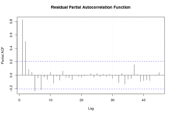
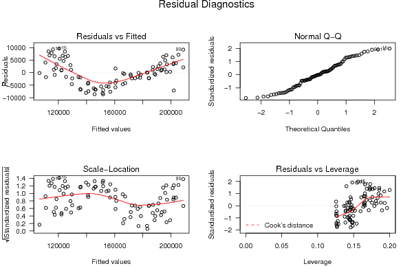
Ws 7 link 3 verbetering

Dataseries X:

» Textbox « » Textfile « » CSV «

106370 100.3 109375 101.9 116476 102.1 123297 103.2 114813 103.7 117925 106.2 126466 107.7 131235 109.9 120546 111.7 123791 114.9 129813 116 133463 118.3 122987 120.4 125418 126 130199 128.1 133016 130.1 121454 130.8 122044 133.6 128313 134.2 131556 135.5 120027 136.2 123001 139.1 130111 139 132524 139.6 123742 138.7 124931 140.9 133646 141.3 136557 141.8 127509 142 128945 144.5 137191 144.6 139716 145.5 129083 146.8 131604 149.5 139413 149.9 143125 150.1 133948 150.9 137116 152.8 144864 153.1 149277 154 138796 154.9 143258 156.9 150034 158.4 154708 159.7 144888 160.2 148762 163.2 156500 163.7 161088 164.4 152772 163.7 158011 165.5 163318 165.6 169969 166.8 162269 167.5 165765 170.6 170600 170.9 174681 172 166364 171.8 170240 173.9 176150 174 182056 173.8 172218 173.9 177856 176 182253 176.6 188090 178.2 176863 179.2 183273 181.3 187969 181.8 194650 182.9 183036 183.8 189516 186.3 193805 187.4 200499 189.2 188142 189.7 193732 191.9 1971 etc...

Output produced by software:

Enter (or paste) a matrix (table) containing all data (time) series. Every column represents a different variable and must be delimited by a space or Tab. Every row represents a period in time (or category) and must be delimited by hard returns. The easiest way to enter data is to copy and paste a block of spreadsheet cells. Please, do not use commas or spaces to seperate groups of digits! Summary of computational transaction Raw Input view raw input (R code) Raw Output view raw output of R engine Computing time 10 seconds R Server 'Gwilym Jenkins' @ 72.249.127.135 Multiple Linear Regression - Estimated Regression Equation Y[t] = + 208567.107938821 -921.004563567302X[t] -11949.1975185385M1[t] -8082.79076424465M2[t] -3965.65512368413M3[t] -343.269483123576M4[t] -13602.4626075061M5[t] -7617.86920888109M6[t] -4314.85008049639M7[t] -468.345557023851M8[t] -12413.4718215697M9[t] -8127.28954572532M10[t] -3619.37471336142M11[t] + 2261.93056733788t + e[t] Multiple Linear Regression - Ordinary Least Squares Variable Parameter S.D. T-STAT H0: parameter = 0 2-tail p-value 1-tail p-value (Intercept) 208567.107938821 16132.48965 12.9284 0 0 X -921.004563567302 150.601916 -6.1155 0 0 M1 -11949.1975185385 2732.774495 -4.3726 3.8e-05 1.9e-05 M2 -8082.79076424465 2722.398061 -2.969 0.003995 0.001998 M3 -3965.65512368413 2722.493331 -1.4566 0.149339 0.074669 M4 -343.269483123576 2723.995504 -0.126 0.900051 0.450026 M5 -13602.4626075061 2737.786077 -4.9684 4e-06 2e-06 M6 -7617.86920888109 2723.022221 -2.7976 0.00652 0.00326 M7 -4314.85008049639 2815.653101 -1.5325 0.129564 0.064782 M8 -468.345557023851 2813.448906 -0.1665 0.868232 0.434116 M9 -12413.4718215697 2814.539857 -4.4105 3.3e-05 1.7e-05 M10 -8127.28954572532 2812.493631 -2.8897 0.005023 0.002511 M11 -3619.37471336142 2810.379633 -1.2879 0.201702 0.100851 t 2261.93056733788 181.715335 12.4477 0 0 Multiple Linear Regression - Regression Statistics Multiple R 0.987784594200056 R-squared 0.97571840453897 Adjusted R-squared 0.971564973736425 F-TEST (value) 234.918661445175 F-TEST (DF numerator) 13 F-TEST (DF denominator) 76 p-value 0 Multiple Linear Regression - Residual Statistics Residual Standard Deviation 5257.57399585094 Sum Squared Residuals 2100798408.46045 Multiple Linear Regression - Actuals, Interpolation, and Residuals Time or Index Actuals Interpolation Forecast Residuals Prediction Error 1 106370 106503.083261820 -133.083261819800 2 109375 111157.813281744 -1782.81328174364 3 116476 117352.678576929 -876.678576928715 4 123297 122223.889764903 1073.11023509688 5 114813 110766.124926075 4046.87507392511 6 117925 116710.137483119 1214.86251688052 7 126466 120893.580333491 5572.41966650889 8 131235 124975.805384453 6259.19461554652 9 120546 113634.801472824 6911.19852717565 10 123791 117235.699712591 6555.30028740875 11 129813 122992.440092369 6820.559907631 12 133463 126755.434876864 6707.56512313648 13 122987 115134.058342172 7852.94165782846 14 125418 116104.770107826 9313.22989217358 15 130199 120549.726732233 9649.2732677665 16 133016 124592.033812997 8423.96618700268 17 121454 112950.068061456 8503.9319385444 18 122044 118617.77924943 3426.22075056998 19 128313 123630.126207012 4682.87379298777 20 131556 128541.255365185 3014.74463481485 21 120027 118213.35647348 1813.64352651992 22 123001 122090.556082317 910.443917682825 23 130111 128952.501938376 1158.49806162433 24 132524 134281.204480935 -1757.20448093461 25 123742 125422.841636945 -1680.84163694455 26 124931 129524.968918728 -4593.96891872821 27 133646 135535.633301200 -1889.63330119970 28 136557 140959.447227314 -4402.44722731448 29 127509 129777.983757556 -2268.98375755644 30 128945 135721.996314601 -6776.99631460102 31 137191 141194.845553967 -4003.8455539669 32 139716 146474.376537567 -6758.37653756674 33 129083 135593.874907721 -6510.87490772127 34 131604 139655.275429272 -8051.27542927183 35 139413 146056.719003547 -6643.71900354668 36 143125 151753.823371533 -8628.82337153254 37 133948 141329.752769478 -7381.75276947805 38 137116 145708.181420332 -8592.18142033193 39 144864 151810.946259160 -6946.94625916016 40 149277 156866.358359848 -7589.35835984802 41 138796 145040.191695593 -6244.19169559285 42 143258 151444.706534421 -8186.7065344211 43 150034 155628.149384793 -5594.14938479273 44 154708 160539.278542966 -5831.27854296567 45 144888 150395.580563974 -5507.58056397406 46 148762 154180.679716454 -5418.67971645442 47 156500 160490.022834373 -3990.02283437255 48 161088 165726.624920575 -4638.62492057473 49 152772 156684.061163871 -3912.06116387121 50 158011 161154.590271082 -3143.59027108181 51 163318 167441.556022623 -4123.5560226235 52 169969 172220.666754241 -2251.66675424115 53 162269 160578.701002699 1690.29899730054 54 165765 165970.110821604 -205.110821603674 55 170600 171258.759148256 -658.759148256062 56 174681 176354.089219142 -1673.08921914246 57 166364 166855.094434648 -491.094434647949 58 170240 171469.097694339 -1229.09769433888 59 176150 178146.842637684 -1996.84263768394 60 182056 184212.348831097 -2156.34883109670 61 172218 174432.981423539 -2214.98142353933 62 177856 178627.209161680 -771.20916167975 63 182253 184453.672631438 -2200.67263143779 64 188090 188864.381537629 -774.381537628538 65 176863 176946.114417017 -83.1144170166443 66 183273 183258.528799488 14.4712005118637 67 187969 188362.976213427 -393.976213427077 68 194650 193458.306284313 1191.69371568653 69 183036 182946.206479895 89.7935201050704 70 189516 187191.807914159 2324.19208584106 71 193805 192948.548293937 856.45170606331 72 200499 197172.045360215 3326.95463978512 73 188142 187024.276127231 1117.72387276941 74 193732 191126.403409014 2605.59659098575 75 197126 196860.766422416 265.233577584431 76 205140 201731.97761039 3408.02238961003 77 191751 190274.212771562 1476.78722843826 78 196700 195389.321221396 1310.67877860426 79 199784 199388.563159054 395.436840946102 80 207360 203562.888666373 3797.11133362698 81 196101 192406.085667457 3694.91433254264 82 200824 195914.883450868 4909.11654913249 83 205743 201947.925199715 3795.07480028453 84 212489 205342.518158783 7146.48184121697 85 200810 194457.945274945 6352.05472505507 86 203683 196718.063429594 6964.936570406 87 207286 201163.020054001 6122.97994599892 88 210910 208797.244932677 2112.75506732260 89 194915 202036.603368042 -7121.60336804239 90 217920 208717.419575941 9202.58042405917 Goldfeld-Quandt test for Heteroskedasticity p-values Alternative Hypothesis breakpoint index greater 2-sided less 17 0.211206215985269 0.422412431970538 0.788793784014731 18 0.261014386253473 0.522028772506947 0.738985613746527 19 0.491143328333681 0.982286656667362 0.508856671666319 20 0.770710092712927 0.458579814574147 0.229289907287073 21 0.937407333735248 0.125185332529505 0.0625926662647524 22 0.980813494645118 0.0383730107097632 0.0191865053548816 23 0.99418939688302 0.0116212062339602 0.00581060311698009 24 0.997586513246027 0.00482697350794683 0.00241348675397342 25 0.997371015430165 0.00525796913966987 0.00262898456983494 26 0.995784305096446 0.00843138980710884 0.00421569490355442 27 0.996447837044364 0.00710432591127247 0.00355216295563623 28 0.995253664870073 0.00949267025985409 0.00474633512992704 29 0.997464778069645 0.00507044386070992 0.00253522193035496 30 0.9954695031813 0.00906099363739892 0.00453049681869946 31 0.994871283163326 0.0102574336733486 0.00512871683667431 32 0.991494230999957 0.0170115380000860 0.00850576900004298 33 0.986260677957435 0.0274786440851295 0.0137393220425647 34 0.979064584296247 0.0418708314075065 0.0209354157037532 35 0.967906554934248 0.0641868901315044 0.0320934450657522 36 0.958243792759204 0.083512414481591 0.0417562072407955 37 0.951711425125311 0.0965771497493778 0.0482885748746889 38 0.95486724596435 0.0902655080713021 0.0451327540356511 39 0.948638493008892 0.102723013982215 0.0513615069911076 40 0.942046454467135 0.115907091065730 0.0579535455328648 41 0.925890233430573 0.148219533138855 0.0741097665694274 42 0.94710931422156 0.105781371556878 0.0528906857784389 43 0.936378482024093 0.127243035951813 0.0636215179759065 44 0.9357729797013 0.128454040597399 0.0642270202986997 45 0.937039656324475 0.125920687351049 0.0629603436755247 46 0.949150474807711 0.101699050384577 0.0508495251922886 47 0.949449759433212 0.101100481133577 0.0505502405667884 48 0.966008804038021 0.0679823919239577 0.0339911959619789 49 0.975737971285994 0.0485240574280111 0.0242620287140056 50 0.98600654091514 0.0279869181697210 0.0139934590848605 51 0.985886386853033 0.028227226293933 0.0141136131469665 52 0.986720966333837 0.0265580673323266 0.0132790336661633 53 0.996965878211644 0.00606824357671248 0.00303412178835624 54 0.997432846607075 0.00513430678585079 0.00256715339292539 55 0.996815108740522 0.006369782518956 0.003184891259478 56 0.995605207188998 0.00878958562200451 0.00439479281100225 57 0.993946412046476 0.0121071759070481 0.00605358795352404 58 0.991930276846118 0.0161394463077644 0.00806972315388218 59 0.987503161516327 0.0249936769673457 0.0124968384836728 60 0.98738564485686 0.0252287102862821 0.0126143551431411 61 0.98327942536772 0.0334411492645586 0.0167205746322793 62 0.977658332888707 0.0446833342225855 0.0223416671112928 63 0.966046111064364 0.0679077778712726 0.0339538889356363 64 0.947795942752344 0.104408114495312 0.0522040572476562 65 0.94851762683861 0.102964746322781 0.0514823731613903 66 0.934219970627858 0.131560058744284 0.0657800293721418 67 0.893716893260073 0.212566213479854 0.106283106739927 68 0.839877595372661 0.320244809254678 0.160122404627339 69 0.765102352424426 0.469795295151148 0.234897647575574 70 0.671839603637274 0.656320792725453 0.328160396362726 71 0.549230760608345 0.90153847878331 0.450769239391655 72 0.430518651947018 0.861037303894036 0.569481348052982 73 0.308003549494393 0.616007098988787 0.691996450505607 Meta Analysis of Goldfeld-Quandt test for Heteroskedasticity Description # significant tests % significant tests OK/NOK 1% type I error level 11 0.192982456140351 NOK 5% type I error level 27 0.473684210526316 NOK 10% type I error level 33 0.578947368421053 NOK

Charts produced by software:

http://www.freestatistics.org/blog/date/2009/Nov/22/t1258927458uk4erilyx1pk3u2/107y821258927376.png (open in new window) http://www.freestatistics.org/blog/date/2009/Nov/22/t1258927458uk4erilyx1pk3u2/107y821258927376.ps (open in new window) http://www.freestatistics.org/blog/date/2009/Nov/22/t1258927458uk4erilyx1pk3u2/1tbf01258927376.png (open in new window) http://www.freestatistics.org/blog/date/2009/Nov/22/t1258927458uk4erilyx1pk3u2/1tbf01258927376.ps (open in new window) http://www.freestatistics.org/blog/date/2009/Nov/22/t1258927458uk4erilyx1pk3u2/2g68f1258927376.png (open in new window) http://www.freestatistics.org/blog/date/2009/Nov/22/t1258927458uk4erilyx1pk3u2/2g68f1258927376.ps (open in new window) http://www.freestatistics.org/blog/date/2009/Nov/22/t1258927458uk4erilyx1pk3u2/3a3691258927376.png (open in new window) http://www.freestatistics.org/blog/date/2009/Nov/22/t1258927458uk4erilyx1pk3u2/3a3691258927376.ps (open in new window) http://www.freestatistics.org/blog/date/2009/Nov/22/t1258927458uk4erilyx1pk3u2/4pks61258927376.png (open in new window) http://www.freestatistics.org/blog/date/2009/Nov/22/t1258927458uk4erilyx1pk3u2/4pks61258927376.ps (open in new window) http://www.freestatistics.org/blog/date/2009/Nov/22/t1258927458uk4erilyx1pk3u2/5p0q01258927376.png (open in new window) http://www.freestatistics.org/blog/date/2009/Nov/22/t1258927458uk4erilyx1pk3u2/5p0q01258927376.ps (open in new window) http://www.freestatistics.org/blog/date/2009/Nov/22/t1258927458uk4erilyx1pk3u2/6k3vp1258927376.png (open in new window) http://www.freestatistics.org/blog/date/2009/Nov/22/t1258927458uk4erilyx1pk3u2/6k3vp1258927376.ps (open in new window) http://www.freestatistics.org/blog/date/2009/Nov/22/t1258927458uk4erilyx1pk3u2/748a51258927376.png (open in new window) http://www.freestatistics.org/blog/date/2009/Nov/22/t1258927458uk4erilyx1pk3u2/748a51258927376.ps (open in new window) http://www.freestatistics.org/blog/date/2009/Nov/22/t1258927458uk4erilyx1pk3u2/8b3cd1258927376.png (open in new window) http://www.freestatistics.org/blog/date/2009/Nov/22/t1258927458uk4erilyx1pk3u2/8b3cd1258927376.ps (open in new window) http://www.freestatistics.org/blog/date/2009/Nov/22/t1258927458uk4erilyx1pk3u2/9ceqn1258927376.png (open in new window) http://www.freestatistics.org/blog/date/2009/Nov/22/t1258927458uk4erilyx1pk3u2/9ceqn1258927376.ps (open in new window)

Parameters (Session):

par1 = 1 ; par2 = Include Monthly Dummies ; par3 = Linear Trend ;

Parameters (R input):

par1 = 1 ; par2 = Include Monthly Dummies ; par3 = Linear Trend ;

R code (references can be found in the software module):

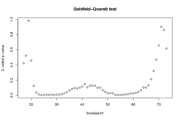
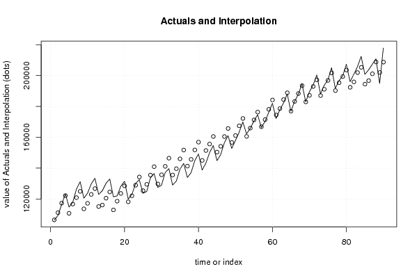
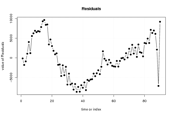
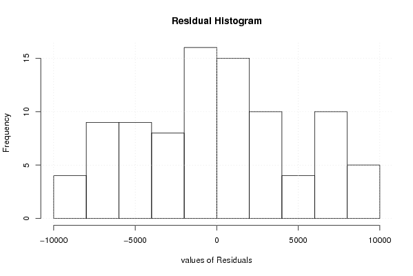
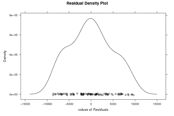
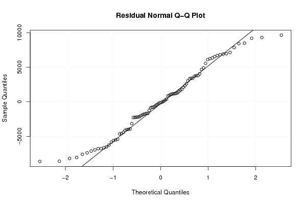
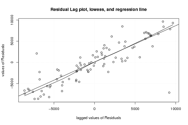
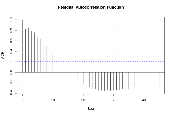
library(lattice) library(lmtest) n25 <- 25 #minimum number of obs. for Goldfeld-Quandt test par1 <- as.numeric(par1) x <- t(y) k <- length(x[1,]) n <- length(x[,1]) x1 <- cbind(x[,par1], x[,1:k!=par1]) mycolnames <- c(colnames(x)[par1], colnames(x)[1:k!=par1]) colnames(x1) <- mycolnames #colnames(x)[par1] x <- x1 if (par3 == 'First Differences'){ x2 <- array(0, dim=c(n-1,k), dimnames=list(1:(n-1), paste('(1-B)',colnames(x),sep=''))) for (i in 1:n-1) { for (j in 1:k) { x2[i,j] <- x[i+1,j] - x[i,j] } } x <- x2 } if (par2 == 'Include Monthly Dummies'){ x2 <- array(0, dim=c(n,11), dimnames=list(1:n, paste('M', seq(1:11), sep =''))) for (i in 1:11){ x2[seq(i,n,12),i] <- 1 } x <- cbind(x, x2) } if (par2 == 'Include Quarterly Dummies'){ x2 <- array(0, dim=c(n,3), dimnames=list(1:n, paste('Q', seq(1:3), sep =''))) for (i in 1:3){ x2[seq(i,n,4),i] <- 1 } x <- cbind(x, x2) } k <- length(x[1,]) if (par3 == 'Linear Trend'){ x <- cbind(x, c(1:n)) colnames(x)[k+1] <- 't' } x k <- length(x[1,]) df <- as.data.frame(x) (mylm <- lm(df)) (mysum <- summary(mylm)) if (n > n25) { kp3 <- k + 3 nmkm3 <- n - k - 3 gqarr <- array(NA, dim=c(nmkm3-kp3+1,3)) numgqtests <- 0 numsignificant1 <- 0 numsignificant5 <- 0 numsignificant10 <- 0 for (mypoint in kp3:nmkm3) { j <- 0 numgqtests <- numgqtests + 1 for (myalt in c('greater', 'two.sided', 'less')) { j <- j + 1 gqarr[mypoint-kp3+1,j] <- gqtest(mylm, point=mypoint, alternative=myalt)$p.value } if (gqarr[mypoint-kp3+1,2] < 0.01) numsignificant1 <- numsignificant1 + 1 if (gqarr[mypoint-kp3+1,2] < 0.05) numsignificant5 <- numsignificant5 + 1 if (gqarr[mypoint-kp3+1,2] < 0.10) numsignificant10 <- numsignificant10 + 1 } gqarr } bitmap(file='test0.png') plot(x[,1], type='l', main='Actuals and Interpolation', ylab='value of Actuals and Interpolation (dots)', xlab='time or index') points(x[,1]-mysum$resid) grid() dev.off() bitmap(file='test1.png') plot(mysum$resid, type='b', pch=19, main='Residuals', ylab='value of Residuals', xlab='time or index') grid() dev.off() bitmap(file='test2.png') hist(mysum$resid, main='Residual Histogram', xlab='values of Residuals') grid() dev.off() bitmap(file='test3.png') densityplot(~mysum$resid,col='black',main='Residual Density Plot', xlab='values of Residuals') dev.off() bitmap(file='test4.png') qqnorm(mysum$resid, main='Residual Normal Q-Q Plot') qqline(mysum$resid) grid() dev.off() (myerror <- as.ts(mysum$resid)) bitmap(file='test5.png') dum <- cbind(lag(myerror,k=1),myerror) dum dum1 <- dum[2:length(myerror),] dum1 z <- as.data.frame(dum1) z plot(z,main=paste('Residual Lag plot, lowess, and regression line'), ylab='values of Residuals', xlab='lagged values of Residuals') lines(lowess(z)) abline(lm(z)) grid() dev.off() bitmap(file='test6.png') acf(mysum$resid, lag.max=length(mysum$resid)/2, main='Residual Autocorrelation Function') grid() dev.off() bitmap(file='test7.png') pacf(mysum$resid, lag.max=length(mysum$resid)/2, main='Residual Partial Autocorrelation Function') grid() dev.off() bitmap(file='test8.png') opar <- par(mfrow = c(2,2), oma = c(0, 0, 1.1, 0)) plot(mylm, las = 1, sub='Residual Diagnostics') par(opar) dev.off() if (n > n25) { bitmap(file='test9.png') plot(kp3:nmkm3,gqarr[,2], main='Goldfeld-Quandt test',ylab='2-sided p-value',xlab='breakpoint') grid() dev.off() } load(file='createtable') a<-table.start() a<-table.row.start(a) a<-table.element(a, 'Multiple Linear Regression - Estimated Regression Equation', 1, TRUE) a<-table.row.end(a) myeq <- colnames(x)[1] myeq <- paste(myeq, '[t] = ', sep='') for (i in 1:k){ if (mysum$coefficients[i,1] > 0) myeq <- paste(myeq, '+', '') myeq <- paste(myeq, mysum$coefficients[i,1], sep=' ') if (rownames(mysum$coefficients)[i] != '(Intercept)') { myeq <- paste(myeq, rownames(mysum$coefficients)[i], sep='') if (rownames(mysum$coefficients)[i] != 't') myeq <- paste(myeq, '[t]', sep='') } } myeq <- paste(myeq, ' + e[t]') a<-table.row.start(a) a<-table.element(a, myeq) a<-table.row.end(a) a<-table.end(a) table.save(a,file='mytable1.tab') a<-table.start() a<-table.row.start(a) a<-table.element(a,hyperlink('http://www.xycoon.com/ols1.htm','Multiple Linear Regression - Ordinary Least Squares',''), 6, TRUE) a<-table.row.end(a) a<-table.row.start(a) a<-table.element(a,'Variable',header=TRUE) a<-table.element(a,'Parameter',header=TRUE) a<-table.element(a,'S.D.',header=TRUE) a<-table.element(a,'T-STAT<br />H0: parameter = 0',header=TRUE) a<-table.element(a,'2-tail p-value',header=TRUE) a<-table.element(a,'1-tail p-value',header=TRUE) a<-table.row.end(a) for (i in 1:k){ a<-table.row.start(a) a<-table.element(a,rownames(mysum$coefficients)[i],header=TRUE) a<-table.element(a,mysum$coefficients[i,1]) a<-table.element(a, round(mysum$coefficients[i,2],6)) a<-table.element(a, round(mysum$coefficients[i,3],4)) a<-table.element(a, round(mysum$coefficients[i,4],6)) a<-table.element(a, round(mysum$coefficients[i,4]/2,6)) a<-table.row.end(a) } a<-table.end(a) table.save(a,file='mytable2.tab') a<-table.start() a<-table.row.start(a) a<-table.element(a, 'Multiple Linear Regression - Regression Statistics', 2, TRUE) a<-table.row.end(a) a<-table.row.start(a) a<-table.element(a, 'Multiple R',1,TRUE) a<-table.element(a, sqrt(mysum$r.squared)) a<-table.row.end(a) a<-table.row.start(a) a<-table.element(a, 'R-squared',1,TRUE) a<-table.element(a, mysum$r.squared) a<-table.row.end(a) a<-table.row.start(a) a<-table.element(a, 'Adjusted R-squared',1,TRUE) a<-table.element(a, mysum$adj.r.squared) a<-table.row.end(a) a<-table.row.start(a) a<-table.element(a, 'F-TEST (value)',1,TRUE) a<-table.element(a, mysum$fstatistic[1]) a<-table.row.end(a) a<-table.row.start(a) a<-table.element(a, 'F-TEST (DF numerator)',1,TRUE) a<-table.element(a, mysum$fstatistic[2]) a<-table.row.end(a) a<-table.row.start(a) a<-table.element(a, 'F-TEST (DF denominator)',1,TRUE) a<-table.element(a, mysum$fstatistic[3]) a<-table.row.end(a) a<-table.row.start(a) a<-table.element(a, 'p-value',1,TRUE) a<-table.element(a, 1-pf(mysum$fstatistic[1],mysum$fstatistic[2],mysum$fstatistic[3])) a<-table.row.end(a) a<-table.row.start(a) a<-table.element(a, 'Multiple Linear Regression - Residual Statistics', 2, TRUE) a<-table.row.end(a) a<-table.row.start(a) a<-table.element(a, 'Residual Standard Deviation',1,TRUE) a<-table.element(a, mysum$sigma) a<-table.row.end(a) a<-table.row.start(a) a<-table.element(a, 'Sum Squared Residuals',1,TRUE) a<-table.element(a, sum(myerror*myerror)) a<-table.row.end(a) a<-table.end(a) table.save(a,file='mytable3.tab') a<-table.start() a<-table.row.start(a) a<-table.element(a, 'Multiple Linear Regression - Actuals, Interpolation, and Residuals', 4, TRUE) a<-table.row.end(a) a<-table.row.start(a) a<-table.element(a, 'Time or Index', 1, TRUE) a<-table.element(a, 'Actuals', 1, TRUE) a<-table.element(a, 'Interpolation<br />Forecast', 1, TRUE) a<-table.element(a, 'Residuals<br />Prediction Error', 1, TRUE) a<-table.row.end(a) for (i in 1:n) { a<-table.row.start(a) a<-table.element(a,i, 1, TRUE) a<-table.element(a,x[i]) a<-table.element(a,x[i]-mysum$resid[i]) a<-table.element(a,mysum$resid[i]) a<-table.row.end(a) } a<-table.end(a) table.save(a,file='mytable4.tab') if (n > n25) { a<-table.start() a<-table.row.start(a) a<-table.element(a,'Goldfeld-Quandt test for Heteroskedasticity',4,TRUE) a<-table.row.end(a) a<-table.row.start(a) a<-table.element(a,'p-values',header=TRUE) a<-table.element(a,'Alternative Hypothesis',3,header=TRUE) a<-table.row.end(a) a<-table.row.start(a) a<-table.element(a,'breakpoint index',header=TRUE) a<-table.element(a,'greater',header=TRUE) a<-table.element(a,'2-sided',header=TRUE) a<-table.element(a,'less',header=TRUE) a<-table.row.end(a) for (mypoint in kp3:nmkm3) { a<-table.row.start(a) a<-table.element(a,mypoint,header=TRUE) a<-table.element(a,gqarr[mypoint-kp3+1,1]) a<-table.element(a,gqarr[mypoint-kp3+1,2]) a<-table.element(a,gqarr[mypoint-kp3+1,3]) a<-table.row.end(a) } a<-table.end(a) table.save(a,file='mytable5.tab') a<-table.start() a<-table.row.start(a) a<-table.element(a,'Meta Analysis of Goldfeld-Quandt test for Heteroskedasticity',4,TRUE) a<-table.row.end(a) a<-table.row.start(a) a<-table.element(a,'Description',header=TRUE) a<-table.element(a,'# significant tests',header=TRUE) a<-table.element(a,'% significant tests',header=TRUE) a<-table.element(a,'OK/NOK',header=TRUE) a<-table.row.end(a) a<-table.row.start(a) a<-table.element(a,'1% type I error level',header=TRUE) a<-table.element(a,numsignificant1) a<-table.element(a,numsignificant1/numgqtests) if (numsignificant1/numgqtests < 0.01) dum <- 'OK' else dum <- 'NOK' a<-table.element(a,dum) a<-table.row.end(a) a<-table.row.start(a) a<-table.element(a,'5% type I error level',header=TRUE) a<-table.element(a,numsignificant5) a<-table.element(a,numsignificant5/numgqtests) if (numsignificant5/numgqtests < 0.05) dum <- 'OK' else dum <- 'NOK' a<-table.element(a,dum) a<-table.row.end(a) a<-table.row.start(a) a<-table.element(a,'10% type I error level',header=TRUE) a<-table.element(a,numsignificant10) a<-table.element(a,numsignificant10/numgqtests) if (numsignificant10/numgqtests < 0.1) dum <- 'OK' else dum <- 'NOK' a<-table.element(a,dum) a<-table.row.end(a) a<-table.end(a) table.save(a,file='mytable6.tab') }

Copyright

This work is licensed under a Creative Commons Attribution-Noncommercial-Share Alike 3.0 License.

Software written by Ed van Stee & Patrick Wessa

Disclaimer

Information provided on this web site is provided "AS IS" without warranty of any kind, either express or implied, including, without limitation, warranties of merchantability, fitness for a particular purpose, and noninfringement. We use reasonable efforts to include accurate and timely information and periodically update the information, and software without notice. However, we make no warranties or representations as to the accuracy or completeness of such information (or software), and we assume no liability or responsibility for errors or omissions in the content of this web site, or any software bugs in online applications. Your use of this web site is AT YOUR OWN RISK. Under no circumstances and under no legal theory shall we be liable to you or any other person for any direct, indirect, special, incidental, exemplary, or consequential damages arising from your access to, or use of, this web site.

Privacy Policy

We may request personal information to be submitted to our servers in order to be able to:

• personalize online software applications according to your needs
• enforce strict security rules with respect to the data that you upload (e.g. statistical data)
• manage user sessions of online applications
• alert you about important changes or upgrades in resources or applications

We NEVER allow other companies to directly offer registered users information about their products and services. Banner references and hyperlinks of third parties NEVER contain any personal data of the visitor.

We do NOT sell, nor transmit by any means, personal information, nor statistical data series uploaded by you to third parties.

We carefully protect your data from loss, misuse, alteration, and destruction. However, at any time, and under any circumstance you are solely responsible for managing your passwords, and keeping them secret.

We store a unique ANONYMOUS USER ID in the form of a small 'Cookie' on your computer. This allows us to track your progress when using this website which is necessary to create state-dependent features. The cookie is used for NO OTHER PURPOSE. At any time you may opt to disallow cookies from this website - this will not affect other features of this website.

We examine cookies that are used by third-parties (banner and online ads) very closely: abuse from third-parties automatically results in termination of the advertising contract without refund. We have very good reason to believe that the cookies that are produced by third parties (banner ads) do NOT cause any privacy or security risk.

FreeStatistics.org is safe. There is no need to download any software to use the applications and services contained in this website. Hence, your system's security is not compromised by their use, and your personal data - other than data you submit in the account application form, and the user-agent information that is transmitted by your browser - is never transmitted to our servers.

As a general rule, we do not log on-line behavior of individuals (other than normal logging of webserver 'hits'). However, in cases of abuse, hacking, unauthorized access, Denial of Service attacks, illegal copying, hotlinking, non-compliance with international webstandards (such as robots.txt), or any other harmful behavior, our system engineers are empowered to log, track, identify, publish, and ban misbehaving individuals - even if this leads to ban entire blocks of IP addresses, or disclosing user's identity.

FreeStatistics.org is powered by