Mutiple Regression Model 1

*The author of this computation has been verified*

R Software Module: /rwasp_multipleregression.wasp (opens new window with default values)

Title produced by software: Multiple Regression

Date of computation: Sat, 21 Nov 2009 09:36:19 -0700

Cite this page as follows:

Statistical Computations at FreeStatistics.org, Office for Research Development and Education, URL http://www.freestatistics.org/blog/date/2009/Nov/21/t1258821621nhkvym6cwvbsdi1.htm/, Retrieved Sat, 21 Nov 2009 17:40:34 +0100

BibTeX entries for LaTeX users:

@Manual{KEY, author = {{YOUR NAME}}, publisher = {Office for Research Development and Education}, title = {Statistical Computations at FreeStatistics.org, URL http://www.freestatistics.org/blog/date/2009/Nov/21/t1258821621nhkvym6cwvbsdi1.htm/}, year = {2009}, } @Manual{R, title = {R: A Language and Environment for Statistical Computing}, author = {{R Development Core Team}}, organization = {R Foundation for Statistical Computing}, address = {Vienna, Austria}, year = {2009}, note = {{ISBN} 3-900051-07-0}, url = {http://www.R-project.org}, }

Original text written by user:

IsPrivate?

No (this computation is public)

User-defined keywords:

KVN WS7

Dataseries X:

» Textbox « » Textfile « » CSV «

9487 1169 8700 2154 9627 2249 8947 2687 9283 4359 8829 5382 9947 4459 9628 6398 9318 4596 9605 3024 8640 1887 9214 2070 9567 1351 8547 2218 9185 2461 9470 3028 9123 4784 9278 4975 10170 4607 9434 6249 9655 4809 9429 3157 8739 1910 9552 2228 9687 1594 9019 2467 9672 2222 9206 3607 9069 4685 9788 4962 10312 5770 10105 5480 9863 5000 9656 3228 9295 1993 9946 2288 9701 1580 9049 2111 10190 2192 9706 3601 9765 4665 9893 4876 9994 5813 10433 5589 10073 5331 10112 3075 9266 2002 9820 2306 10097 1507 9115 1992 10411 2487 9678 3490 10408 4647 10153 5594 10368 5611 10581 5788 10597 6204 10680 3013 9738 1931 9556 2549

Output produced by software:

Enter (or paste) a matrix (table) containing all data (time) series. Every column represents a different variable and must be delimited by a space or Tab. Every row represents a period in time (or category) and must be delimited by hard returns. The easiest way to enter data is to copy and paste a block of spreadsheet cells. Please, do not use commas or spaces to seperate groups of digits! Summary of computational transaction Raw Input view raw input (R code) Raw Output view raw output of R engine Computing time 3 seconds R Server 'Gwilym Jenkins' @ 72.249.127.135 Multiple Linear Regression - Estimated Regression Equation Y[t] = + 9169.31167219994 + 0.132189485048809X[t] + e[t] Multiple Linear Regression - Ordinary Least Squares Variable Parameter S.D. T-STAT H0: parameter = 0 2-tail p-value 1-tail p-value (Intercept) 9169.31167219994 156.733887 58.5024 0 0 X 0.132189485048809 0.040454 3.2676 0.001825 0.000913 Multiple Linear Regression - Regression Statistics Multiple R 0.394297381050267 R-squared 0.155470424703100 Adjusted R-squared 0.140909569956602 F-TEST (value) 10.6772869731764 F-TEST (DF numerator) 1 F-TEST (DF denominator) 58 p-value 0.00182506844110497 Multiple Linear Regression - Residual Statistics Residual Standard Deviation 480.708461588437 Sum Squared Residuals 13402676.2524779 Multiple Linear Regression - Actuals, Interpolation, and Residuals Time or Index Actuals Interpolation Forecast Residuals Prediction Error 1 9487 9323.84118022197 163.158819778034 2 8700 9454.04782299507 -754.047822995071 3 9627 9466.6058240747 160.394175925292 4 8947 9524.5048185261 -577.504818526087 5 9283 9745.5256375277 -462.525637527695 6 8829 9880.75548073263 -1051.75548073263 7 9947 9758.74458603258 188.255413967424 8 9628 10015.0599975422 -387.059997542216 9 9318 9776.85454548426 -458.854545484263 10 9605 9569.05267498754 35.9473250124646 11 8640 9418.75323048704 -778.753230487040 12 9214 9442.94390625097 -228.943906250972 13 9567 9347.89966650088 219.100333499122 14 8547 9462.5079500382 -915.507950038195 15 9185 9494.62999490506 -309.629994905056 16 9470 9569.58143292773 -99.5814329277306 17 9123 9801.70616867344 -678.706168673439 18 9278 9826.95436031776 -548.954360317761 19 10170 9778.3086298198 391.6913701802 20 9434 9995.36376426994 -561.363764269944 21 9655 9805.01090579966 -150.010905799659 22 9429 9586.63387649903 -157.633876499027 23 8739 9421.79358864316 -682.793588643162 24 9552 9463.82984488868 88.1701551113165 25 9687 9380.02171136774 306.978288632261 26 9019 9495.42313181535 -476.423131815349 27 9672 9463.0367079784 208.963292021609 28 9206 9646.119144771 -440.119144770991 29 9069 9788.6194096536 -719.619409653607 30 9788 9825.23589701213 -37.2358970121269 31 10312 9932.04500093156 379.954999068436 32 10105 9893.7100502674 211.28994973259 33 9863 9830.25909744398 32.7409025560184 34 9656 9596.0193299375 59.9806700625076 35 9295 9432.76531590221 -137.765315902213 36 9946 9471.76121399161 474.238786008388 37 9701 9378.17105857706 322.828941422945 38 9049 9448.36367513797 -399.363675137973 39 10190 9459.07102342693 730.928976573074 40 9706 9645.3260078607 60.6739921393019 41 9765 9785.97561995263 -20.9756199526307 42 9893 9813.86760129793 79.1323987020707 43 9994 9937.72914878866 56.2708512113368 44 10433 9908.11870413773 524.88129586227 45 10073 9874.01381699514 198.986183004863 46 10112 9575.79433872503 536.205661274975 47 9266 9433.95502126765 -167.955021267653 48 9820 9474.1406247225 345.859375277509 49 10097 9368.5212261685 728.478773831508 50 9115 9432.63312641716 -317.633126417165 51 10411 9498.06692151633 912.933078483675 52 9678 9630.65297502028 47.3470249797197 53 10408 9783.59620922175 624.403790778248 54 10153 9908.77965156297 244.220348437026 55 10368 9911.0268728088 456.973127191196 56 10581 9934.42441166244 646.575588337557 57 10597 9989.41523744275 607.584762557252 58 10680 9567.598590652 1112.40140934800 59 9738 9424.56956782919 313.430432170813 60 9556 9506.26266958935 49.7373304106488 Goldfeld-Quandt test for Heteroskedasticity p-values Alternative Hypothesis breakpoint index greater 2-sided less 5 0.520024565042372 0.959950869915256 0.479975434957628 6 0.413724024984696 0.827448049969392 0.586275975015304 7 0.661243835537153 0.677512328925694 0.338756164462847 8 0.587016202927084 0.825967594145832 0.412983797072916 9 0.482464645144695 0.96492929028939 0.517535354855305 10 0.411859672250569 0.823719344501137 0.588140327749431 11 0.502427024862969 0.995145950274062 0.497572975137031 12 0.405784691481656 0.811569382963312 0.594215308518344 13 0.372644628662585 0.745289257325171 0.627355371337415 14 0.536554036502045 0.92689192699591 0.463445963497955 15 0.461861774681994 0.923723549363988 0.538138225318006 16 0.396669807604278 0.793339615208556 0.603330192395722 17 0.395448630448552 0.790897260897105 0.604551369551448 18 0.369880901712198 0.739761803424395 0.630119098287802 19 0.517026177001387 0.965947645997225 0.482973822998613 20 0.516477728411952 0.967044543176095 0.483522271588048 21 0.473413666689208 0.946827333378416 0.526586333310792 22 0.415247975937138 0.830495951874276 0.584752024062862 23 0.508558711940513 0.982882576118974 0.491441288059487 24 0.468084566000883 0.936169132001765 0.531915433999117 25 0.463386047843997 0.926772095687993 0.536613952156003 26 0.487922686708008 0.975845373416016 0.512077313291992 27 0.458060784739126 0.916121569478252 0.541939215260874 28 0.481037248673957 0.962074497347913 0.518962751326044 29 0.666844942574584 0.666310114850831 0.333155057425416 30 0.659109793826536 0.681780412346927 0.340890206173464 31 0.716443302338143 0.567113395323714 0.283556697661857 32 0.70517621031988 0.58964757936024 0.29482378968012 33 0.67718053967767 0.645638920644661 0.322819460322331 34 0.635747556359451 0.728504887281098 0.364252443640549 35 0.611940454334625 0.77611909133075 0.388059545665375 36 0.621932725640307 0.756134548719387 0.378067274359693 37 0.580165425237931 0.839669149524137 0.419834574762069 38 0.671278625920834 0.657442748158333 0.328721374079166 39 0.746706528174881 0.506586943650238 0.253293471825119 40 0.70815347136769 0.583693057264619 0.291846528632310 41 0.690670271017836 0.618659457964328 0.309329728982164 42 0.661262914926733 0.677474170146534 0.338737085073267 43 0.654671536616108 0.690656926767784 0.345328463383892 44 0.631809386074003 0.736381227851993 0.368190613925997 45 0.592133024453662 0.815733951092676 0.407866975546338 46 0.55442395741187 0.891152085176258 0.445576042588129 47 0.574043472438038 0.851913055123925 0.425956527561962 48 0.494135921177512 0.988271842355025 0.505864078822488 49 0.515443510637443 0.969112978725114 0.484556489362557 50 0.671253719935094 0.657492560129812 0.328746280064906 51 0.747168156517286 0.505663686965428 0.252831843482714 52 0.738137096636022 0.523725806727956 0.261862903363978 53 0.648373947399488 0.703252105201023 0.351626052600512 54 0.578532003747075 0.84293599250585 0.421467996252925 55 0.440088993341877 0.880177986683753 0.559911006658123 Meta Analysis of Goldfeld-Quandt test for Heteroskedasticity Description # significant tests % significant tests OK/NOK 1% type I error level 0 0 OK 5% type I error level 0 0 OK 10% type I error level 0 0 OK

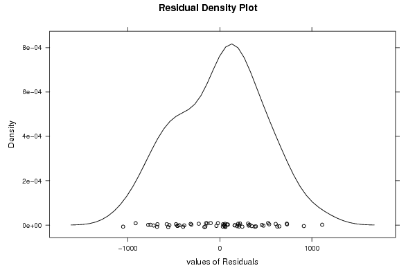
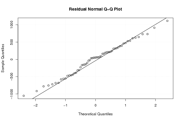
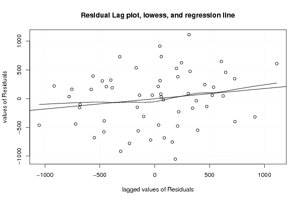
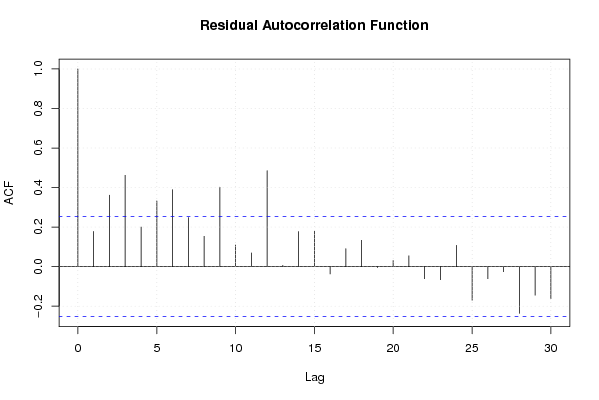
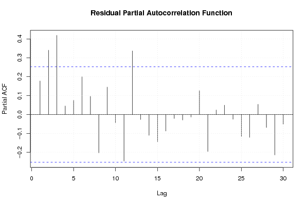
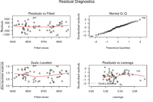
Charts produced by software:

http://www.freestatistics.org/blog/date/2009/Nov/21/t1258821621nhkvym6cwvbsdi1/10u8gs1258821374.png (open in new window) http://www.freestatistics.org/blog/date/2009/Nov/21/t1258821621nhkvym6cwvbsdi1/10u8gs1258821374.ps (open in new window) http://www.freestatistics.org/blog/date/2009/Nov/21/t1258821621nhkvym6cwvbsdi1/155c11258821374.png (open in new window) http://www.freestatistics.org/blog/date/2009/Nov/21/t1258821621nhkvym6cwvbsdi1/155c11258821374.ps (open in new window) http://www.freestatistics.org/blog/date/2009/Nov/21/t1258821621nhkvym6cwvbsdi1/2bio41258821374.png (open in new window) http://www.freestatistics.org/blog/date/2009/Nov/21/t1258821621nhkvym6cwvbsdi1/2bio41258821374.ps (open in new window) http://www.freestatistics.org/blog/date/2009/Nov/21/t1258821621nhkvym6cwvbsdi1/3umns1258821374.png (open in new window) http://www.freestatistics.org/blog/date/2009/Nov/21/t1258821621nhkvym6cwvbsdi1/3umns1258821374.ps (open in new window) http://www.freestatistics.org/blog/date/2009/Nov/21/t1258821621nhkvym6cwvbsdi1/49jto1258821374.png (open in new window) http://www.freestatistics.org/blog/date/2009/Nov/21/t1258821621nhkvym6cwvbsdi1/49jto1258821374.ps (open in new window) http://www.freestatistics.org/blog/date/2009/Nov/21/t1258821621nhkvym6cwvbsdi1/5qh6b1258821374.png (open in new window) http://www.freestatistics.org/blog/date/2009/Nov/21/t1258821621nhkvym6cwvbsdi1/5qh6b1258821374.ps (open in new window) http://www.freestatistics.org/blog/date/2009/Nov/21/t1258821621nhkvym6cwvbsdi1/6synm1258821374.png (open in new window) http://www.freestatistics.org/blog/date/2009/Nov/21/t1258821621nhkvym6cwvbsdi1/6synm1258821374.ps (open in new window) http://www.freestatistics.org/blog/date/2009/Nov/21/t1258821621nhkvym6cwvbsdi1/74ur61258821374.png (open in new window) http://www.freestatistics.org/blog/date/2009/Nov/21/t1258821621nhkvym6cwvbsdi1/74ur61258821374.ps (open in new window) http://www.freestatistics.org/blog/date/2009/Nov/21/t1258821621nhkvym6cwvbsdi1/8mfyr1258821374.png (open in new window) http://www.freestatistics.org/blog/date/2009/Nov/21/t1258821621nhkvym6cwvbsdi1/8mfyr1258821374.ps (open in new window) http://www.freestatistics.org/blog/date/2009/Nov/21/t1258821621nhkvym6cwvbsdi1/91r031258821374.png (open in new window) http://www.freestatistics.org/blog/date/2009/Nov/21/t1258821621nhkvym6cwvbsdi1/91r031258821374.ps (open in new window)

Parameters (Session):

par1 = 1 ; par2 = Do not include Seasonal Dummies ; par3 = No Linear Trend ;

Parameters (R input):

par1 = 1 ; par2 = Do not include Seasonal Dummies ; par3 = No Linear Trend ;

R code (references can be found in the software module):

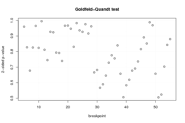
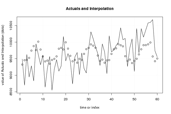
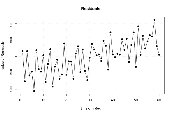
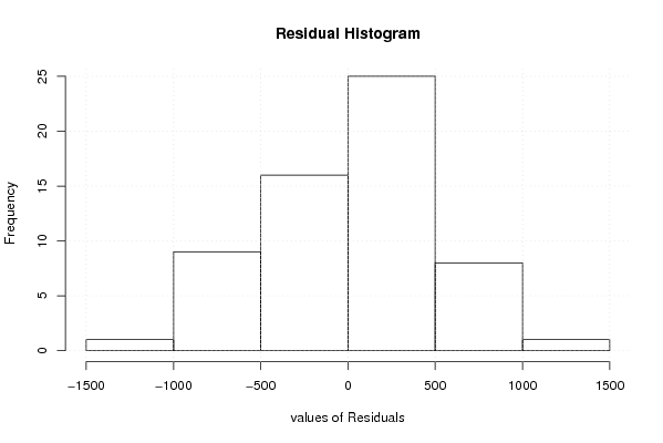
library(lattice) library(lmtest) n25 <- 25 #minimum number of obs. for Goldfeld-Quandt test par1 <- as.numeric(par1) x <- t(y) k <- length(x[1,]) n <- length(x[,1]) x1 <- cbind(x[,par1], x[,1:k!=par1]) mycolnames <- c(colnames(x)[par1], colnames(x)[1:k!=par1]) colnames(x1) <- mycolnames #colnames(x)[par1] x <- x1 if (par3 == 'First Differences'){ x2 <- array(0, dim=c(n-1,k), dimnames=list(1:(n-1), paste('(1-B)',colnames(x),sep=''))) for (i in 1:n-1) { for (j in 1:k) { x2[i,j] <- x[i+1,j] - x[i,j] } } x <- x2 } if (par2 == 'Include Monthly Dummies'){ x2 <- array(0, dim=c(n,11), dimnames=list(1:n, paste('M', seq(1:11), sep =''))) for (i in 1:11){ x2[seq(i,n,12),i] <- 1 } x <- cbind(x, x2) } if (par2 == 'Include Quarterly Dummies'){ x2 <- array(0, dim=c(n,3), dimnames=list(1:n, paste('Q', seq(1:3), sep =''))) for (i in 1:3){ x2[seq(i,n,4),i] <- 1 } x <- cbind(x, x2) } k <- length(x[1,]) if (par3 == 'Linear Trend'){ x <- cbind(x, c(1:n)) colnames(x)[k+1] <- 't' } x k <- length(x[1,]) df <- as.data.frame(x) (mylm <- lm(df)) (mysum <- summary(mylm)) if (n > n25) { kp3 <- k + 3 nmkm3 <- n - k - 3 gqarr <- array(NA, dim=c(nmkm3-kp3+1,3)) numgqtests <- 0 numsignificant1 <- 0 numsignificant5 <- 0 numsignificant10 <- 0 for (mypoint in kp3:nmkm3) { j <- 0 numgqtests <- numgqtests + 1 for (myalt in c('greater', 'two.sided', 'less')) { j <- j + 1 gqarr[mypoint-kp3+1,j] <- gqtest(mylm, point=mypoint, alternative=myalt)$p.value } if (gqarr[mypoint-kp3+1,2] < 0.01) numsignificant1 <- numsignificant1 + 1 if (gqarr[mypoint-kp3+1,2] < 0.05) numsignificant5 <- numsignificant5 + 1 if (gqarr[mypoint-kp3+1,2] < 0.10) numsignificant10 <- numsignificant10 + 1 } gqarr } bitmap(file='test0.png') plot(x[,1], type='l', main='Actuals and Interpolation', ylab='value of Actuals and Interpolation (dots)', xlab='time or index') points(x[,1]-mysum$resid) grid() dev.off() bitmap(file='test1.png') plot(mysum$resid, type='b', pch=19, main='Residuals', ylab='value of Residuals', xlab='time or index') grid() dev.off() bitmap(file='test2.png') hist(mysum$resid, main='Residual Histogram', xlab='values of Residuals') grid() dev.off() bitmap(file='test3.png') densityplot(~mysum$resid,col='black',main='Residual Density Plot', xlab='values of Residuals') dev.off() bitmap(file='test4.png') qqnorm(mysum$resid, main='Residual Normal Q-Q Plot') qqline(mysum$resid) grid() dev.off() (myerror <- as.ts(mysum$resid)) bitmap(file='test5.png') dum <- cbind(lag(myerror,k=1),myerror) dum dum1 <- dum[2:length(myerror),] dum1 z <- as.data.frame(dum1) z plot(z,main=paste('Residual Lag plot, lowess, and regression line'), ylab='values of Residuals', xlab='lagged values of Residuals') lines(lowess(z)) abline(lm(z)) grid() dev.off() bitmap(file='test6.png') acf(mysum$resid, lag.max=length(mysum$resid)/2, main='Residual Autocorrelation Function') grid() dev.off() bitmap(file='test7.png') pacf(mysum$resid, lag.max=length(mysum$resid)/2, main='Residual Partial Autocorrelation Function') grid() dev.off() bitmap(file='test8.png') opar <- par(mfrow = c(2,2), oma = c(0, 0, 1.1, 0)) plot(mylm, las = 1, sub='Residual Diagnostics') par(opar) dev.off() if (n > n25) { bitmap(file='test9.png') plot(kp3:nmkm3,gqarr[,2], main='Goldfeld-Quandt test',ylab='2-sided p-value',xlab='breakpoint') grid() dev.off() } load(file='createtable') a<-table.start() a<-table.row.start(a) a<-table.element(a, 'Multiple Linear Regression - Estimated Regression Equation', 1, TRUE) a<-table.row.end(a) myeq <- colnames(x)[1] myeq <- paste(myeq, '[t] = ', sep='') for (i in 1:k){ if (mysum$coefficients[i,1] > 0) myeq <- paste(myeq, '+', '') myeq <- paste(myeq, mysum$coefficients[i,1], sep=' ') if (rownames(mysum$coefficients)[i] != '(Intercept)') { myeq <- paste(myeq, rownames(mysum$coefficients)[i], sep='') if (rownames(mysum$coefficients)[i] != 't') myeq <- paste(myeq, '[t]', sep='') } } myeq <- paste(myeq, ' + e[t]') a<-table.row.start(a) a<-table.element(a, myeq) a<-table.row.end(a) a<-table.end(a) table.save(a,file='mytable1.tab') a<-table.start() a<-table.row.start(a) a<-table.element(a,hyperlink('http://www.xycoon.com/ols1.htm','Multiple Linear Regression - Ordinary Least Squares',''), 6, TRUE) a<-table.row.end(a) a<-table.row.start(a) a<-table.element(a,'Variable',header=TRUE) a<-table.element(a,'Parameter',header=TRUE) a<-table.element(a,'S.D.',header=TRUE) a<-table.element(a,'T-STAT<br />H0: parameter = 0',header=TRUE) a<-table.element(a,'2-tail p-value',header=TRUE) a<-table.element(a,'1-tail p-value',header=TRUE) a<-table.row.end(a) for (i in 1:k){ a<-table.row.start(a) a<-table.element(a,rownames(mysum$coefficients)[i],header=TRUE) a<-table.element(a,mysum$coefficients[i,1]) a<-table.element(a, round(mysum$coefficients[i,2],6)) a<-table.element(a, round(mysum$coefficients[i,3],4)) a<-table.element(a, round(mysum$coefficients[i,4],6)) a<-table.element(a, round(mysum$coefficients[i,4]/2,6)) a<-table.row.end(a) } a<-table.end(a) table.save(a,file='mytable2.tab') a<-table.start() a<-table.row.start(a) a<-table.element(a, 'Multiple Linear Regression - Regression Statistics', 2, TRUE) a<-table.row.end(a) a<-table.row.start(a) a<-table.element(a, 'Multiple R',1,TRUE) a<-table.element(a, sqrt(mysum$r.squared)) a<-table.row.end(a) a<-table.row.start(a) a<-table.element(a, 'R-squared',1,TRUE) a<-table.element(a, mysum$r.squared) a<-table.row.end(a) a<-table.row.start(a) a<-table.element(a, 'Adjusted R-squared',1,TRUE) a<-table.element(a, mysum$adj.r.squared) a<-table.row.end(a) a<-table.row.start(a) a<-table.element(a, 'F-TEST (value)',1,TRUE) a<-table.element(a, mysum$fstatistic[1]) a<-table.row.end(a) a<-table.row.start(a) a<-table.element(a, 'F-TEST (DF numerator)',1,TRUE) a<-table.element(a, mysum$fstatistic[2]) a<-table.row.end(a) a<-table.row.start(a) a<-table.element(a, 'F-TEST (DF denominator)',1,TRUE) a<-table.element(a, mysum$fstatistic[3]) a<-table.row.end(a) a<-table.row.start(a) a<-table.element(a, 'p-value',1,TRUE) a<-table.element(a, 1-pf(mysum$fstatistic[1],mysum$fstatistic[2],mysum$fstatistic[3])) a<-table.row.end(a) a<-table.row.start(a) a<-table.element(a, 'Multiple Linear Regression - Residual Statistics', 2, TRUE) a<-table.row.end(a) a<-table.row.start(a) a<-table.element(a, 'Residual Standard Deviation',1,TRUE) a<-table.element(a, mysum$sigma) a<-table.row.end(a) a<-table.row.start(a) a<-table.element(a, 'Sum Squared Residuals',1,TRUE) a<-table.element(a, sum(myerror*myerror)) a<-table.row.end(a) a<-table.end(a) table.save(a,file='mytable3.tab') a<-table.start() a<-table.row.start(a) a<-table.element(a, 'Multiple Linear Regression - Actuals, Interpolation, and Residuals', 4, TRUE) a<-table.row.end(a) a<-table.row.start(a) a<-table.element(a, 'Time or Index', 1, TRUE) a<-table.element(a, 'Actuals', 1, TRUE) a<-table.element(a, 'Interpolation<br />Forecast', 1, TRUE) a<-table.element(a, 'Residuals<br />Prediction Error', 1, TRUE) a<-table.row.end(a) for (i in 1:n) { a<-table.row.start(a) a<-table.element(a,i, 1, TRUE) a<-table.element(a,x[i]) a<-table.element(a,x[i]-mysum$resid[i]) a<-table.element(a,mysum$resid[i]) a<-table.row.end(a) } a<-table.end(a) table.save(a,file='mytable4.tab') if (n > n25) { a<-table.start() a<-table.row.start(a) a<-table.element(a,'Goldfeld-Quandt test for Heteroskedasticity',4,TRUE) a<-table.row.end(a) a<-table.row.start(a) a<-table.element(a,'p-values',header=TRUE) a<-table.element(a,'Alternative Hypothesis',3,header=TRUE) a<-table.row.end(a) a<-table.row.start(a) a<-table.element(a,'breakpoint index',header=TRUE) a<-table.element(a,'greater',header=TRUE) a<-table.element(a,'2-sided',header=TRUE) a<-table.element(a,'less',header=TRUE) a<-table.row.end(a) for (mypoint in kp3:nmkm3) { a<-table.row.start(a) a<-table.element(a,mypoint,header=TRUE) a<-table.element(a,gqarr[mypoint-kp3+1,1]) a<-table.element(a,gqarr[mypoint-kp3+1,2]) a<-table.element(a,gqarr[mypoint-kp3+1,3]) a<-table.row.end(a) } a<-table.end(a) table.save(a,file='mytable5.tab') a<-table.start() a<-table.row.start(a) a<-table.element(a,'Meta Analysis of Goldfeld-Quandt test for Heteroskedasticity',4,TRUE) a<-table.row.end(a) a<-table.row.start(a) a<-table.element(a,'Description',header=TRUE) a<-table.element(a,'# significant tests',header=TRUE) a<-table.element(a,'% significant tests',header=TRUE) a<-table.element(a,'OK/NOK',header=TRUE) a<-table.row.end(a) a<-table.row.start(a) a<-table.element(a,'1% type I error level',header=TRUE) a<-table.element(a,numsignificant1) a<-table.element(a,numsignificant1/numgqtests) if (numsignificant1/numgqtests < 0.01) dum <- 'OK' else dum <- 'NOK' a<-table.element(a,dum) a<-table.row.end(a) a<-table.row.start(a) a<-table.element(a,'5% type I error level',header=TRUE) a<-table.element(a,numsignificant5) a<-table.element(a,numsignificant5/numgqtests) if (numsignificant5/numgqtests < 0.05) dum <- 'OK' else dum <- 'NOK' a<-table.element(a,dum) a<-table.row.end(a) a<-table.row.start(a) a<-table.element(a,'10% type I error level',header=TRUE) a<-table.element(a,numsignificant10) a<-table.element(a,numsignificant10/numgqtests) if (numsignificant10/numgqtests < 0.1) dum <- 'OK' else dum <- 'NOK' a<-table.element(a,dum) a<-table.row.end(a) a<-table.end(a) table.save(a,file='mytable6.tab') }

Copyright

This work is licensed under a Creative Commons Attribution-Noncommercial-Share Alike 3.0 License.

Software written by Ed van Stee & Patrick Wessa

Disclaimer

Information provided on this web site is provided "AS IS" without warranty of any kind, either express or implied, including, without limitation, warranties of merchantability, fitness for a particular purpose, and noninfringement. We use reasonable efforts to include accurate and timely information and periodically update the information, and software without notice. However, we make no warranties or representations as to the accuracy or completeness of such information (or software), and we assume no liability or responsibility for errors or omissions in the content of this web site, or any software bugs in online applications. Your use of this web site is AT YOUR OWN RISK. Under no circumstances and under no legal theory shall we be liable to you or any other person for any direct, indirect, special, incidental, exemplary, or consequential damages arising from your access to, or use of, this web site.

Privacy Policy

We may request personal information to be submitted to our servers in order to be able to:

• personalize online software applications according to your needs
• enforce strict security rules with respect to the data that you upload (e.g. statistical data)
• manage user sessions of online applications
• alert you about important changes or upgrades in resources or applications

We NEVER allow other companies to directly offer registered users information about their products and services. Banner references and hyperlinks of third parties NEVER contain any personal data of the visitor.

We do NOT sell, nor transmit by any means, personal information, nor statistical data series uploaded by you to third parties.

We carefully protect your data from loss, misuse, alteration, and destruction. However, at any time, and under any circumstance you are solely responsible for managing your passwords, and keeping them secret.

We store a unique ANONYMOUS USER ID in the form of a small 'Cookie' on your computer. This allows us to track your progress when using this website which is necessary to create state-dependent features. The cookie is used for NO OTHER PURPOSE. At any time you may opt to disallow cookies from this website - this will not affect other features of this website.

We examine cookies that are used by third-parties (banner and online ads) very closely: abuse from third-parties automatically results in termination of the advertising contract without refund. We have very good reason to believe that the cookies that are produced by third parties (banner ads) do NOT cause any privacy or security risk.

FreeStatistics.org is safe. There is no need to download any software to use the applications and services contained in this website. Hence, your system's security is not compromised by their use, and your personal data - other than data you submit in the account application form, and the user-agent information that is transmitted by your browser - is never transmitted to our servers.

As a general rule, we do not log on-line behavior of individuals (other than normal logging of webserver 'hits'). However, in cases of abuse, hacking, unauthorized access, Denial of Service attacks, illegal copying, hotlinking, non-compliance with international webstandards (such as robots.txt), or any other harmful behavior, our system engineers are empowered to log, track, identify, publish, and ban misbehaving individuals - even if this leads to ban entire blocks of IP addresses, or disclosing user's identity.

FreeStatistics.org is powered by