ws7

*The author of this computation has been verified*

R Software Module: /rwasp_multipleregression.wasp (opens new window with default values)

Title produced by software: Multiple Regression

Date of computation: Wed, 18 Nov 2009 12:32:58 -0700

Cite this page as follows:

Statistical Computations at FreeStatistics.org, Office for Research Development and Education, URL http://www.freestatistics.org/blog/date/2009/Nov/18/t125857287910fc31bzdlxl6ti.htm/, Retrieved Wed, 18 Nov 2009 20:34:51 +0100

BibTeX entries for LaTeX users:

@Manual{KEY, author = {{YOUR NAME}}, publisher = {Office for Research Development and Education}, title = {Statistical Computations at FreeStatistics.org, URL http://www.freestatistics.org/blog/date/2009/Nov/18/t125857287910fc31bzdlxl6ti.htm/}, year = {2009}, } @Manual{R, title = {R: A Language and Environment for Statistical Computing}, author = {{R Development Core Team}}, organization = {R Foundation for Statistical Computing}, address = {Vienna, Austria}, year = {2009}, note = {{ISBN} 3-900051-07-0}, url = {http://www.R-project.org}, }

Original text written by user:

IsPrivate?

No (this computation is public)

User-defined keywords:

Dataseries X:

» Textbox « » Textfile « » CSV «

216234 562325 213587 560854 209465 555332 204045 543599 200237 536662 203666 542722 241476 593530 260307 610763 243324 612613 244460 611324 233575 594167 237217 595454 235243 590865 230354 589379 227184 584428 221678 573100 217142 567456 219452 569028 256446 620735 265845 628884 248624 628232 241114 612117 229245 595404 231805 597141 219277 593408 219313 590072 212610 579799 214771 574205 211142 572775 211457 572942 240048 619567 240636 625809 230580 619916 208795 587625 197922 565742 194596 557274 194581 560576 185686 548854 178106 531673 172608 525919 167302 511038 168053 498662 202300 555362 202388 564591 182516 541657 173476 527070 166444 509846 171297 514258 169701 516922 164182 507561 161914 492622 159612 490243 151001 469357 158114 477580 186530 528379 187069 533590 174330 517945 169362 506174 166827 501866 178037 516141 186412 528222 189226 532638 191563 536322 188906 536535 186005 523597 195309 536214 223532 586570 226899 596594 2141 etc...

Output produced by software:

Enter (or paste) a matrix (table) containing all data (time) series. Every column represents a different variable and must be delimited by a space or Tab. Every row represents a period in time (or category) and must be delimited by hard returns. The easiest way to enter data is to copy and paste a block of spreadsheet cells. Please, do not use commas or spaces to seperate groups of digits! Summary of computational transaction Raw Input view raw input (R code) Raw Output view raw output of R engine Computing time 5 seconds R Server 'Gwilym Jenkins' @ 72.249.127.135 Multiple Linear Regression - Estimated Regression Equation Y[t] = -133727.514270307 + 0.618935182546662X[t] -1755.19220226771M1[t] -2352.19962173868M2[t] -645.253981753101M3[t] + 141.872350504839M4[t] + 2030.7627839215M5[t] + 4441.33958694601M6[t] + 5371.03914127785M7[t] + 5271.76700348223M8[t] -3329.24764649524M9[t] -3512.30395609849M10[t] -2366.35555749082M11[t] -217.867281983915t + e[t] Multiple Linear Regression - Ordinary Least Squares Variable Parameter S.D. T-STAT H0: parameter = 0 2-tail p-value 1-tail p-value (Intercept) -133727.514270307 18975.798968 -7.0473 0 0 X 0.618935182546662 0.031189 19.8447 0 0 M1 -1755.19220226771 4023.176626 -0.4363 0.664348 0.332174 M2 -2352.19962173868 4024.298764 -0.5845 0.561275 0.280637 M3 -645.253981753101 4038.840255 -0.1598 0.873654 0.436827 M4 141.872350504839 4055.963372 0.035 0.972223 0.486112 M5 2030.7627839215 4104.956622 0.4947 0.622775 0.311388 M6 4441.33958694601 4081.407123 1.0882 0.281258 0.140629 M7 5371.03914127785 4118.695273 1.3041 0.197643 0.098822 M8 5271.76700348223 4204.167307 1.2539 0.215168 0.107584 M9 -3329.24764649524 4133.399667 -0.8055 0.424029 0.212014 M10 -3512.30395609849 4208.720832 -0.8345 0.407593 0.203796 M11 -2366.35555749082 4197.296154 -0.5638 0.575195 0.287597 t -217.867281983915 54.973963 -3.9631 0.000215 0.000108 Multiple Linear Regression - Regression Statistics Multiple R 0.977991520492774 R-squared 0.956467414155768 Adjusted R-squared 0.946177893865313 F-TEST (value) 92.9554913306353 F-TEST (DF numerator) 13 F-TEST (DF denominator) 55 p-value 0 Multiple Linear Regression - Residual Statistics Residual Standard Deviation 6633.49154690541 Sum Squared Residuals 2420176555.65760 Multiple Linear Regression - Actuals, Interpolation, and Residuals Time or Index Actuals Interpolation Forecast Residuals Prediction Error 1 216234 212342.152770992 3891.84722900816 2 213587 210616.824416011 2970.17558398852 3 209465 208688.142695990 776.857304009579 4 204045 201995.435249444 2049.56475055554 5 200237 199372.905039551 864.094960448992 6 203666 205316.361766824 -1650.36176682438 7 241476 237475.052794003 4000.94720599689 8 260307 247824.02337505 12482.9766249498 9 243324 240150.1715308 3173.82846919986 10 244460 238951.44048891 5508.55951108968 11 233575 229260.450678581 4314.549321419 12 237217 232205.508534025 5011.49146597453 13 235243 227392.155497067 7850.8445029328 14 230354 225657.543114348 4696.45688565202 15 227184 224082.273383561 3101.72661643888 16 221678 217640.234685947 4037.76531405344 17 217142 215817.987667086 1324.01233291406 18 219452 218983.66329509 468.336704910103 19 256446 251698.777051378 4747.22294862193 20 265845 256425.340434171 9419.65956582871 21 248624 247202.912763189 1421.08723681053 22 241114 236827.848704863 4286.15129513716 23 229245 227411.666115584 1833.33388441576 24 231805 230635.244803175 1169.75519682530 25 219277 226351.700282476 -7074.70028247639 26 219313 223472.057812046 -4159.05781204584 27 212610 218602.815039746 -5992.81503974564 28 214771 215709.750678854 -938.750678853642 29 211142 216495.696519245 -5353.69651924466 30 211457 218791.768215771 -7334.76821577055 31 240048 248361.453374357 -8313.45337435659 32 240636 251907.707364033 -11271.7073640333 33 230580 239441.440401324 -8861.44040132445 34 208795 219054.480830123 -10259.4808301230 35 197922 206438.403347078 -8516.40334707818 36 194596 203345.74849678 -8749.74849677994 37 194581 203416.412985297 -8835.4129852974 38 185686 195346.380074031 -9660.38007403054 39 178106 186201.533060698 -8095.533060698 40 172608 183209.439070599 -10601.4390705985 41 167302 175670.087770554 -8368.08777055441 42 168053 170202.855472398 -2149.85547239752 43 202300 206008.312595141 -3708.31259514118 44 202388 211403.325975085 -9015.32597508479 45 182516 188389.784566598 -5873.78456659825 46 173476 178960.453467203 -5484.45346720292 47 166444 169227.994999643 -2783.99499964297 48 171297 174107.225300546 -2810.22530054576 49 169701 173783.009142598 -4082.00914259843 50 164182 167174.282197324 -2992.28219732425 51 161914 159417.087863261 2496.91213673867 52 159612 158513.900114257 1098.09988574315 53 151001 147257.84304302 3743.15695697999 54 158114 154540.056570142 3573.94342985818 55 186530 186693.177180678 -163.177180677613 56 187069 189601.308997149 -2532.30899714874 57 174330 171099.186134245 3230.81386575518 58 169362 163412.776508901 5949.2234910991 59 166827 161674.484859114 5152.51514088637 60 178037 172658.272865474 5378.72713452586 61 186412 178162.569321569 8249.43067843126 62 189226 180080.91238624 9145.08761376009 63 191563 183850.147956743 7712.85204325652 64 188906 184551.2402009 4354.75979910005 65 186005 178214.479960544 7790.52003945602 66 195309 188216.294679776 7092.70532022419 67 223532 220095.227004443 3436.77299555655 68 226899 225982.293854512 916.706145488341 69 214126 207216.504603843 6909.49539615713 Goldfeld-Quandt test for Heteroskedasticity p-values Alternative Hypothesis breakpoint index greater 2-sided less 17 0.00167920821262012 0.00335841642524023 0.99832079178738 18 0.000585165431129338 0.00117033086225868 0.99941483456887 19 0.000227308493920914 0.000454616987841828 0.999772691506079 20 0.000360578867106827 0.000721157734213654 0.999639421132893 21 0.000134074795171082 0.000268149590342163 0.99986592520483 22 0.000471970602669675 0.00094394120533935 0.99952802939733 23 0.000271350906062639 0.000542701812125278 0.999728649093937 24 0.000290814083905192 0.000581628167810384 0.999709185916095 25 0.137208067867088 0.274416135734176 0.862791932132912 26 0.140200941350678 0.280401882701357 0.859799058649322 27 0.101978757575680 0.203957515151359 0.89802124242432 28 0.272156382721353 0.544312765442706 0.727843617278647 29 0.306024681025131 0.612049362050263 0.693975318974869 30 0.252819461907942 0.505638923815884 0.747180538092058 31 0.429895158281292 0.859790316562584 0.570104841718708 32 0.934919066940597 0.130161866118806 0.0650809330594032 33 0.95957185647502 0.08085628704996 0.04042814352498 34 0.963469337754558 0.0730613244908842 0.0365306622454421 35 0.9804826844064 0.0390346311871999 0.0195173155935999 36 0.985596822990192 0.0288063540196155 0.0144031770098077 37 0.987124397917788 0.0257512041644241 0.0128756020822121 38 0.983838924910082 0.032322150179836 0.016161075089918 39 0.986711443460981 0.0265771130780373 0.0132885565390186 40 0.978707546599757 0.0425849068004858 0.0212924534002429 41 0.981124981543497 0.0377500369130055 0.0188750184565027 42 0.992435805105118 0.0151283897897646 0.00756419489488232 43 0.998242768869052 0.00351446226189614 0.00175723113094807 44 0.999290515076174 0.00141896984765277 0.000709484923826384 45 0.999129604895843 0.00174079020831339 0.000870395104156696 46 0.997702279461477 0.00459544107704649 0.00229772053852325 47 0.998358283575135 0.0032834328497299 0.00164171642486495 48 0.99974175071246 0.000516498575078504 0.000258249287539252 49 0.999027217180456 0.00194556563908711 0.000972782819543553 50 0.999976835341899 4.63293162030479e-05 2.31646581015240e-05 51 0.999993230344745 1.35393105103059e-05 6.76965525515294e-06 52 0.999976677212159 4.66455756827535e-05 2.33227878413767e-05 Meta Analysis of Goldfeld-Quandt test for Heteroskedasticity Description # significant tests % significant tests OK/NOK 1% type I error level 18 0.5 NOK 5% type I error level 26 0.722222222222222 NOK 10% type I error level 28 0.777777777777778 NOK

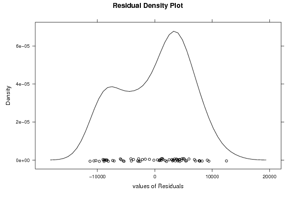
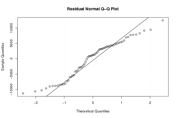
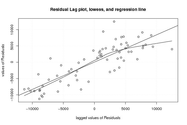
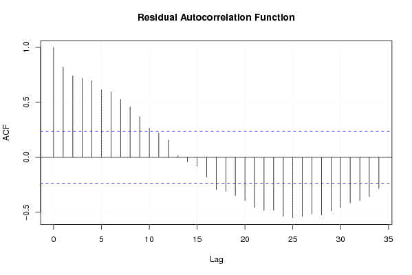
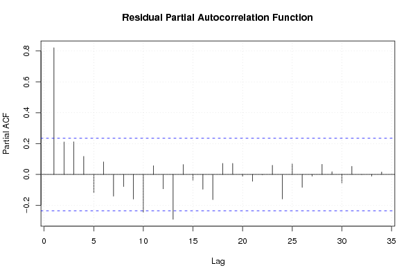
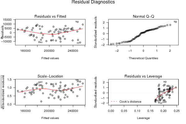
Charts produced by software:

http://www.freestatistics.org/blog/date/2009/Nov/18/t125857287910fc31bzdlxl6ti/10hmrm1258572771.png (open in new window) http://www.freestatistics.org/blog/date/2009/Nov/18/t125857287910fc31bzdlxl6ti/10hmrm1258572771.ps (open in new window) http://www.freestatistics.org/blog/date/2009/Nov/18/t125857287910fc31bzdlxl6ti/15ccb1258572771.png (open in new window) http://www.freestatistics.org/blog/date/2009/Nov/18/t125857287910fc31bzdlxl6ti/15ccb1258572771.ps (open in new window) http://www.freestatistics.org/blog/date/2009/Nov/18/t125857287910fc31bzdlxl6ti/20yt21258572771.png (open in new window) http://www.freestatistics.org/blog/date/2009/Nov/18/t125857287910fc31bzdlxl6ti/20yt21258572771.ps (open in new window) http://www.freestatistics.org/blog/date/2009/Nov/18/t125857287910fc31bzdlxl6ti/3s7wj1258572771.png (open in new window) http://www.freestatistics.org/blog/date/2009/Nov/18/t125857287910fc31bzdlxl6ti/3s7wj1258572771.ps (open in new window) http://www.freestatistics.org/blog/date/2009/Nov/18/t125857287910fc31bzdlxl6ti/4flzk1258572771.png (open in new window) http://www.freestatistics.org/blog/date/2009/Nov/18/t125857287910fc31bzdlxl6ti/4flzk1258572771.ps (open in new window) http://www.freestatistics.org/blog/date/2009/Nov/18/t125857287910fc31bzdlxl6ti/54s9p1258572771.png (open in new window) http://www.freestatistics.org/blog/date/2009/Nov/18/t125857287910fc31bzdlxl6ti/54s9p1258572771.ps (open in new window) http://www.freestatistics.org/blog/date/2009/Nov/18/t125857287910fc31bzdlxl6ti/6jndk1258572771.png (open in new window) http://www.freestatistics.org/blog/date/2009/Nov/18/t125857287910fc31bzdlxl6ti/6jndk1258572771.ps (open in new window) http://www.freestatistics.org/blog/date/2009/Nov/18/t125857287910fc31bzdlxl6ti/7r9p71258572771.png (open in new window) http://www.freestatistics.org/blog/date/2009/Nov/18/t125857287910fc31bzdlxl6ti/7r9p71258572771.ps (open in new window) http://www.freestatistics.org/blog/date/2009/Nov/18/t125857287910fc31bzdlxl6ti/8erbj1258572771.png (open in new window) http://www.freestatistics.org/blog/date/2009/Nov/18/t125857287910fc31bzdlxl6ti/8erbj1258572771.ps (open in new window) http://www.freestatistics.org/blog/date/2009/Nov/18/t125857287910fc31bzdlxl6ti/9fx471258572771.png (open in new window) http://www.freestatistics.org/blog/date/2009/Nov/18/t125857287910fc31bzdlxl6ti/9fx471258572771.ps (open in new window)

Parameters (Session):

par1 = 1 ; par2 = Include Monthly Dummies ; par3 = Linear Trend ;

Parameters (R input):

par1 = 1 ; par2 = Include Monthly Dummies ; par3 = Linear Trend ;

R code (references can be found in the software module):

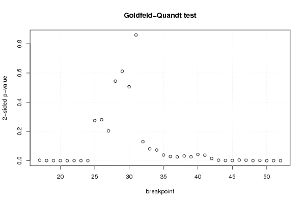
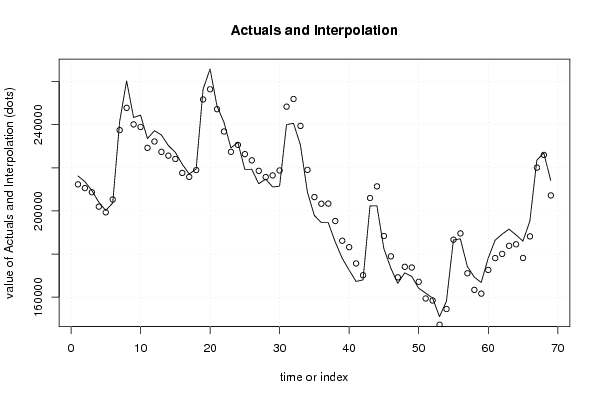
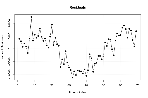
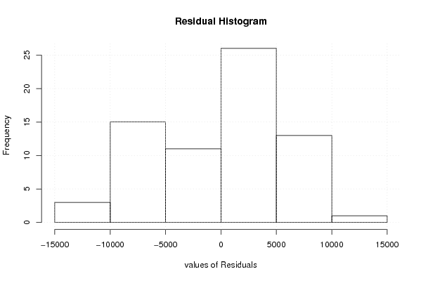
library(lattice) library(lmtest) n25 <- 25 #minimum number of obs. for Goldfeld-Quandt test par1 <- as.numeric(par1) x <- t(y) k <- length(x[1,]) n <- length(x[,1]) x1 <- cbind(x[,par1], x[,1:k!=par1]) mycolnames <- c(colnames(x)[par1], colnames(x)[1:k!=par1]) colnames(x1) <- mycolnames #colnames(x)[par1] x <- x1 if (par3 == 'First Differences'){ x2 <- array(0, dim=c(n-1,k), dimnames=list(1:(n-1), paste('(1-B)',colnames(x),sep=''))) for (i in 1:n-1) { for (j in 1:k) { x2[i,j] <- x[i+1,j] - x[i,j] } } x <- x2 } if (par2 == 'Include Monthly Dummies'){ x2 <- array(0, dim=c(n,11), dimnames=list(1:n, paste('M', seq(1:11), sep =''))) for (i in 1:11){ x2[seq(i,n,12),i] <- 1 } x <- cbind(x, x2) } if (par2 == 'Include Quarterly Dummies'){ x2 <- array(0, dim=c(n,3), dimnames=list(1:n, paste('Q', seq(1:3), sep =''))) for (i in 1:3){ x2[seq(i,n,4),i] <- 1 } x <- cbind(x, x2) } k <- length(x[1,]) if (par3 == 'Linear Trend'){ x <- cbind(x, c(1:n)) colnames(x)[k+1] <- 't' } x k <- length(x[1,]) df <- as.data.frame(x) (mylm <- lm(df)) (mysum <- summary(mylm)) if (n > n25) { kp3 <- k + 3 nmkm3 <- n - k - 3 gqarr <- array(NA, dim=c(nmkm3-kp3+1,3)) numgqtests <- 0 numsignificant1 <- 0 numsignificant5 <- 0 numsignificant10 <- 0 for (mypoint in kp3:nmkm3) { j <- 0 numgqtests <- numgqtests + 1 for (myalt in c('greater', 'two.sided', 'less')) { j <- j + 1 gqarr[mypoint-kp3+1,j] <- gqtest(mylm, point=mypoint, alternative=myalt)$p.value } if (gqarr[mypoint-kp3+1,2] < 0.01) numsignificant1 <- numsignificant1 + 1 if (gqarr[mypoint-kp3+1,2] < 0.05) numsignificant5 <- numsignificant5 + 1 if (gqarr[mypoint-kp3+1,2] < 0.10) numsignificant10 <- numsignificant10 + 1 } gqarr } bitmap(file='test0.png') plot(x[,1], type='l', main='Actuals and Interpolation', ylab='value of Actuals and Interpolation (dots)', xlab='time or index') points(x[,1]-mysum$resid) grid() dev.off() bitmap(file='test1.png') plot(mysum$resid, type='b', pch=19, main='Residuals', ylab='value of Residuals', xlab='time or index') grid() dev.off() bitmap(file='test2.png') hist(mysum$resid, main='Residual Histogram', xlab='values of Residuals') grid() dev.off() bitmap(file='test3.png') densityplot(~mysum$resid,col='black',main='Residual Density Plot', xlab='values of Residuals') dev.off() bitmap(file='test4.png') qqnorm(mysum$resid, main='Residual Normal Q-Q Plot') qqline(mysum$resid) grid() dev.off() (myerror <- as.ts(mysum$resid)) bitmap(file='test5.png') dum <- cbind(lag(myerror,k=1),myerror) dum dum1 <- dum[2:length(myerror),] dum1 z <- as.data.frame(dum1) z plot(z,main=paste('Residual Lag plot, lowess, and regression line'), ylab='values of Residuals', xlab='lagged values of Residuals') lines(lowess(z)) abline(lm(z)) grid() dev.off() bitmap(file='test6.png') acf(mysum$resid, lag.max=length(mysum$resid)/2, main='Residual Autocorrelation Function') grid() dev.off() bitmap(file='test7.png') pacf(mysum$resid, lag.max=length(mysum$resid)/2, main='Residual Partial Autocorrelation Function') grid() dev.off() bitmap(file='test8.png') opar <- par(mfrow = c(2,2), oma = c(0, 0, 1.1, 0)) plot(mylm, las = 1, sub='Residual Diagnostics') par(opar) dev.off() if (n > n25) { bitmap(file='test9.png') plot(kp3:nmkm3,gqarr[,2], main='Goldfeld-Quandt test',ylab='2-sided p-value',xlab='breakpoint') grid() dev.off() } load(file='createtable') a<-table.start() a<-table.row.start(a) a<-table.element(a, 'Multiple Linear Regression - Estimated Regression Equation', 1, TRUE) a<-table.row.end(a) myeq <- colnames(x)[1] myeq <- paste(myeq, '[t] = ', sep='') for (i in 1:k){ if (mysum$coefficients[i,1] > 0) myeq <- paste(myeq, '+', '') myeq <- paste(myeq, mysum$coefficients[i,1], sep=' ') if (rownames(mysum$coefficients)[i] != '(Intercept)') { myeq <- paste(myeq, rownames(mysum$coefficients)[i], sep='') if (rownames(mysum$coefficients)[i] != 't') myeq <- paste(myeq, '[t]', sep='') } } myeq <- paste(myeq, ' + e[t]') a<-table.row.start(a) a<-table.element(a, myeq) a<-table.row.end(a) a<-table.end(a) table.save(a,file='mytable1.tab') a<-table.start() a<-table.row.start(a) a<-table.element(a,hyperlink('http://www.xycoon.com/ols1.htm','Multiple Linear Regression - Ordinary Least Squares',''), 6, TRUE) a<-table.row.end(a) a<-table.row.start(a) a<-table.element(a,'Variable',header=TRUE) a<-table.element(a,'Parameter',header=TRUE) a<-table.element(a,'S.D.',header=TRUE) a<-table.element(a,'T-STAT<br />H0: parameter = 0',header=TRUE) a<-table.element(a,'2-tail p-value',header=TRUE) a<-table.element(a,'1-tail p-value',header=TRUE) a<-table.row.end(a) for (i in 1:k){ a<-table.row.start(a) a<-table.element(a,rownames(mysum$coefficients)[i],header=TRUE) a<-table.element(a,mysum$coefficients[i,1]) a<-table.element(a, round(mysum$coefficients[i,2],6)) a<-table.element(a, round(mysum$coefficients[i,3],4)) a<-table.element(a, round(mysum$coefficients[i,4],6)) a<-table.element(a, round(mysum$coefficients[i,4]/2,6)) a<-table.row.end(a) } a<-table.end(a) table.save(a,file='mytable2.tab') a<-table.start() a<-table.row.start(a) a<-table.element(a, 'Multiple Linear Regression - Regression Statistics', 2, TRUE) a<-table.row.end(a) a<-table.row.start(a) a<-table.element(a, 'Multiple R',1,TRUE) a<-table.element(a, sqrt(mysum$r.squared)) a<-table.row.end(a) a<-table.row.start(a) a<-table.element(a, 'R-squared',1,TRUE) a<-table.element(a, mysum$r.squared) a<-table.row.end(a) a<-table.row.start(a) a<-table.element(a, 'Adjusted R-squared',1,TRUE) a<-table.element(a, mysum$adj.r.squared) a<-table.row.end(a) a<-table.row.start(a) a<-table.element(a, 'F-TEST (value)',1,TRUE) a<-table.element(a, mysum$fstatistic[1]) a<-table.row.end(a) a<-table.row.start(a) a<-table.element(a, 'F-TEST (DF numerator)',1,TRUE) a<-table.element(a, mysum$fstatistic[2]) a<-table.row.end(a) a<-table.row.start(a) a<-table.element(a, 'F-TEST (DF denominator)',1,TRUE) a<-table.element(a, mysum$fstatistic[3]) a<-table.row.end(a) a<-table.row.start(a) a<-table.element(a, 'p-value',1,TRUE) a<-table.element(a, 1-pf(mysum$fstatistic[1],mysum$fstatistic[2],mysum$fstatistic[3])) a<-table.row.end(a) a<-table.row.start(a) a<-table.element(a, 'Multiple Linear Regression - Residual Statistics', 2, TRUE) a<-table.row.end(a) a<-table.row.start(a) a<-table.element(a, 'Residual Standard Deviation',1,TRUE) a<-table.element(a, mysum$sigma) a<-table.row.end(a) a<-table.row.start(a) a<-table.element(a, 'Sum Squared Residuals',1,TRUE) a<-table.element(a, sum(myerror*myerror)) a<-table.row.end(a) a<-table.end(a) table.save(a,file='mytable3.tab') a<-table.start() a<-table.row.start(a) a<-table.element(a, 'Multiple Linear Regression - Actuals, Interpolation, and Residuals', 4, TRUE) a<-table.row.end(a) a<-table.row.start(a) a<-table.element(a, 'Time or Index', 1, TRUE) a<-table.element(a, 'Actuals', 1, TRUE) a<-table.element(a, 'Interpolation<br />Forecast', 1, TRUE) a<-table.element(a, 'Residuals<br />Prediction Error', 1, TRUE) a<-table.row.end(a) for (i in 1:n) { a<-table.row.start(a) a<-table.element(a,i, 1, TRUE) a<-table.element(a,x[i]) a<-table.element(a,x[i]-mysum$resid[i]) a<-table.element(a,mysum$resid[i]) a<-table.row.end(a) } a<-table.end(a) table.save(a,file='mytable4.tab') if (n > n25) { a<-table.start() a<-table.row.start(a) a<-table.element(a,'Goldfeld-Quandt test for Heteroskedasticity',4,TRUE) a<-table.row.end(a) a<-table.row.start(a) a<-table.element(a,'p-values',header=TRUE) a<-table.element(a,'Alternative Hypothesis',3,header=TRUE) a<-table.row.end(a) a<-table.row.start(a) a<-table.element(a,'breakpoint index',header=TRUE) a<-table.element(a,'greater',header=TRUE) a<-table.element(a,'2-sided',header=TRUE) a<-table.element(a,'less',header=TRUE) a<-table.row.end(a) for (mypoint in kp3:nmkm3) { a<-table.row.start(a) a<-table.element(a,mypoint,header=TRUE) a<-table.element(a,gqarr[mypoint-kp3+1,1]) a<-table.element(a,gqarr[mypoint-kp3+1,2]) a<-table.element(a,gqarr[mypoint-kp3+1,3]) a<-table.row.end(a) } a<-table.end(a) table.save(a,file='mytable5.tab') a<-table.start() a<-table.row.start(a) a<-table.element(a,'Meta Analysis of Goldfeld-Quandt test for Heteroskedasticity',4,TRUE) a<-table.row.end(a) a<-table.row.start(a) a<-table.element(a,'Description',header=TRUE) a<-table.element(a,'# significant tests',header=TRUE) a<-table.element(a,'% significant tests',header=TRUE) a<-table.element(a,'OK/NOK',header=TRUE) a<-table.row.end(a) a<-table.row.start(a) a<-table.element(a,'1% type I error level',header=TRUE) a<-table.element(a,numsignificant1) a<-table.element(a,numsignificant1/numgqtests) if (numsignificant1/numgqtests < 0.01) dum <- 'OK' else dum <- 'NOK' a<-table.element(a,dum) a<-table.row.end(a) a<-table.row.start(a) a<-table.element(a,'5% type I error level',header=TRUE) a<-table.element(a,numsignificant5) a<-table.element(a,numsignificant5/numgqtests) if (numsignificant5/numgqtests < 0.05) dum <- 'OK' else dum <- 'NOK' a<-table.element(a,dum) a<-table.row.end(a) a<-table.row.start(a) a<-table.element(a,'10% type I error level',header=TRUE) a<-table.element(a,numsignificant10) a<-table.element(a,numsignificant10/numgqtests) if (numsignificant10/numgqtests < 0.1) dum <- 'OK' else dum <- 'NOK' a<-table.element(a,dum) a<-table.row.end(a) a<-table.end(a) table.save(a,file='mytable6.tab') }

Copyright

This work is licensed under a Creative Commons Attribution-Noncommercial-Share Alike 3.0 License.

Software written by Ed van Stee & Patrick Wessa

Disclaimer

Information provided on this web site is provided "AS IS" without warranty of any kind, either express or implied, including, without limitation, warranties of merchantability, fitness for a particular purpose, and noninfringement. We use reasonable efforts to include accurate and timely information and periodically update the information, and software without notice. However, we make no warranties or representations as to the accuracy or completeness of such information (or software), and we assume no liability or responsibility for errors or omissions in the content of this web site, or any software bugs in online applications. Your use of this web site is AT YOUR OWN RISK. Under no circumstances and under no legal theory shall we be liable to you or any other person for any direct, indirect, special, incidental, exemplary, or consequential damages arising from your access to, or use of, this web site.

Privacy Policy

We may request personal information to be submitted to our servers in order to be able to:

• personalize online software applications according to your needs
• enforce strict security rules with respect to the data that you upload (e.g. statistical data)
• manage user sessions of online applications
• alert you about important changes or upgrades in resources or applications

We NEVER allow other companies to directly offer registered users information about their products and services. Banner references and hyperlinks of third parties NEVER contain any personal data of the visitor.

We do NOT sell, nor transmit by any means, personal information, nor statistical data series uploaded by you to third parties.

We carefully protect your data from loss, misuse, alteration, and destruction. However, at any time, and under any circumstance you are solely responsible for managing your passwords, and keeping them secret.

We store a unique ANONYMOUS USER ID in the form of a small 'Cookie' on your computer. This allows us to track your progress when using this website which is necessary to create state-dependent features. The cookie is used for NO OTHER PURPOSE. At any time you may opt to disallow cookies from this website - this will not affect other features of this website.

We examine cookies that are used by third-parties (banner and online ads) very closely: abuse from third-parties automatically results in termination of the advertising contract without refund. We have very good reason to believe that the cookies that are produced by third parties (banner ads) do NOT cause any privacy or security risk.

FreeStatistics.org is safe. There is no need to download any software to use the applications and services contained in this website. Hence, your system's security is not compromised by their use, and your personal data - other than data you submit in the account application form, and the user-agent information that is transmitted by your browser - is never transmitted to our servers.

As a general rule, we do not log on-line behavior of individuals (other than normal logging of webserver 'hits'). However, in cases of abuse, hacking, unauthorized access, Denial of Service attacks, illegal copying, hotlinking, non-compliance with international webstandards (such as robots.txt), or any other harmful behavior, our system engineers are empowered to log, track, identify, publish, and ban misbehaving individuals - even if this leads to ban entire blocks of IP addresses, or disclosing user's identity.

FreeStatistics.org is powered by